
Utilizing CatBoost Machine Learning model as a Filter for Trend-Following Strategies
Introduction
CatBoost is a powerful tree-based machine learning model that specializes in decision-making based on stationary features. Other tree-based models like XGBoost and Random Forest share similar traits in terms of their robustness, ability to handle complex patterns, and interpretability. These models have a wide range of uses, from feature analysis to risk management.
In this article, we're going to walk through the procedure of utilizing a trained CatBoost model as a filter for a classic moving average cross trend-following strategy. This article is meant to provide insights into the strategy development process while addressing the challenges one may face along the way. I will introduce my workflow of fetching data from MetaTrader 5, training machine learning model in python, and integrating back to MetaTrader 5 expert advisors. By the end of this article, we will validate the strategy through statistical testing and discuss future aspirations extending from the current approach.
Intuition
The rule of thumb in the industry for developing CTA (Commodity Trading Advisor) strategy is that it's best to have a clear, intuitive explanation behind every strategy idea. This is basically how people think of strategy ideas in the first place, not to mention it avoids overfitting as well. This suggestion is subservient even working with machine learning models. We'll try to explain the intuition behind this idea.
Why this could work:
CatBoost model creates decision trees that take in the feature inputs and output the probability of each outcome. In this case, we're only training on binary outcomes (1 is win,0 is loss). The model will alter rules in the decision trees so that it minimizes the loss function in the training data set. If the model displays a certain level of predictability on the out-of-sample testing outcome, we may consider using it to filter out trades that have little probability of winning, which could in turn boost the overall profitability.
A realistic expectation for retail traders like you and I is that the models we train will not be like oracles, but rather only slightly better than random walk. There are plenty of ways to improve the model precision, which I will discuss later, but nevertheless it's a great endeavor for slight improvement.
Optimizing Backbone Strategy
We already know from the above section that we can only expect the model to boost the performance slightly, and thus it's crucial for the backbone strategy to already have some sort of profitability.
The strategy also has to be able to generate abundant samples because:
- The model will filter out a portion of the trades, we want to make sure there are enough samples left to exhibit statistical significance of Laws of Big Numbers.
- We need enough samples for the model to train on so that it minimizes the loss function for in-sample data effectively.
We use a historically proven trend following strategy which takes trades when two moving averages of different period crosses, and we exit trades when the price turns to the opposite side of the moving average. i.e. following the trend. The following MQL5 code is the expert advisor for this strategy.
#include <Trade/Trade.mqh>
//XAU - 1h.
CTrade trade;

input ENUM_TIMEFRAMES TF = PERIOD_CURRENT;
input ENUM_MA_METHOD MaMethod = MODE_SMA;
input ENUM_APPLIED_PRICE MaAppPrice = PRICE_CLOSE;
input int MaPeriodsFast = 15;
input int MaPeriodsSlow = 25;
input int MaPeriods = 200;
input double lott = 0.01;
ulong buypos = 0, sellpos = 0;
input int Magic = 0;
int barsTotal = 0;
int handleMaFast;
int handleMaSlow;
int handleMa;

//+------------------------------------------------------------------+
//| Expert initialization function                                   |
//+------------------------------------------------------------------+
int OnInit()
  {
   trade.SetExpertMagicNumber(Magic);
   handleMaFast =iMA(_Symbol,TF,MaPeriodsFast,0,MaMethod,MaAppPrice);
   handleMaSlow =iMA(_Symbol,TF,MaPeriodsSlow,0,MaMethod,MaAppPrice);
   handleMa = iMA(_Symbol,TF,MaPeriods,0,MaMethod,MaAppPrice);
   return(INIT_SUCCEEDED);
  }

//+------------------------------------------------------------------+
//| Expert deinitialization function                                 |
//+------------------------------------------------------------------+
void OnDeinit(const int reason)
  {

  }

//+------------------------------------------------------------------+
//| Expert tick function                                             |
//+------------------------------------------------------------------+
void OnTick()
  {
  int bars = iBars(_Symbol,PERIOD_CURRENT);
  //Beware, the last element of the buffer list is the most recent data, not [0]
  if (barsTotal!= bars){
     barsTotal = bars;
     double maFast[];
     double maSlow[];
     double ma[];
     CopyBuffer(handleMaFast,BASE_LINE,1,2,maFast);
     CopyBuffer(handleMaSlow,BASE_LINE,1,2,maSlow);
     CopyBuffer(handleMa,0,1,1,ma);
     double bid = SymbolInfoDouble(_Symbol, SYMBOL_BID);
     double ask = SymbolInfoDouble(_Symbol, SYMBOL_ASK);
     double lastClose = iClose(_Symbol, PERIOD_CURRENT, 1);
     //The order below matters
     if(buypos>0&& lastClose<maSlow[1]) trade.PositionClose(buypos);
     if(sellpos>0 &&lastClose>maSlow[1])trade.PositionClose(sellpos);
     if (maFast[1]>maSlow[1]&&maFast[0]<maSlow[0]&&buypos ==sellpos)executeBuy();
     if(maFast[1]<maSlow[1]&&maFast[0]>maSlow[0]&&sellpos ==buypos) executeSell();
     if(buypos>0&&(!PositionSelectByTicket(buypos)|| PositionGetInteger(POSITION_MAGIC) != Magic)){
      buypos = 0;
      }
     if(sellpos>0&&(!PositionSelectByTicket(sellpos)|| PositionGetInteger(POSITION_MAGIC) != Magic)){
      sellpos = 0;
      }
    }
 }

//+------------------------------------------------------------------+
//| Expert trade transaction handling function                       |
//+------------------------------------------------------------------+
void OnTradeTransaction(const MqlTradeTransaction& trans, const MqlTradeRequest& request, const MqlTradeResult& result) {
    if (trans.type == TRADE_TRANSACTION_ORDER_ADD) {
        COrderInfo order;
        if (order.Select(trans.order)) {
            if (order.Magic() == Magic) {
                if (order.OrderType() == ORDER_TYPE_BUY) {
                    buypos = order.Ticket();
                } else if (order.OrderType() == ORDER_TYPE_SELL) {
                    sellpos = order.Ticket();
                }
            }
        }
    }
}

//+------------------------------------------------------------------+
//| Execute sell trade function                                      |
//+------------------------------------------------------------------+
void executeSell() {
       double bid = SymbolInfoDouble(_Symbol, SYMBOL_BID);
       bid = NormalizeDouble(bid,_Digits);
       trade.Sell(lott,_Symbol,bid);
       sellpos = trade.ResultOrder();
       }

//+------------------------------------------------------------------+
//| Execute buy trade function                                       |
//+------------------------------------------------------------------+
void executeBuy() {
       double ask = SymbolInfoDouble(_Symbol, SYMBOL_ASK);
       ask = NormalizeDouble(ask,_Digits);
       trade.Buy(lott,_Symbol,ask);
       buypos = trade.ResultOrder();
}
For validating your backbone strategy, here are a few things to consider:
- Enough sample size (frequency depends on your timeframe and signal restriction, but total samples I suggest 1000-10000. Each trade is a sample.)
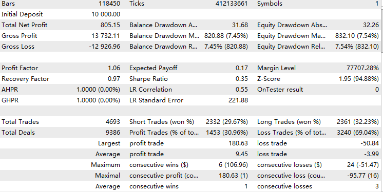
- Already exhibits some sort of profitability but not too much (Profit factor is 1-1.15 I would say is good enough. Because the MetaTrader 5 tester already accounts for spreads, having a profit factor of 1 means it has a statistical edge already. If the profit factor exceeds 1.15, the strategy is most likely good enough to stand on its own, and you probably don't need more filters to increase complexity.)
- The backbone strategy doesn't have too many parameters. (The backbone strategy is better to be simple, since using a machine learning model as a filter already increases plenty of complexity to your strategy. The less filter, the less chance of overfitting.)
These are what I did to optimize the strategy:
- Finding a good timeframe. After running the code in different timeframe, I found that this strategy works best on higher timeframe, but to generate enough samples, I eventually stuck with 1h timeframe.
- Optimizing parameters. I optimized the slow MA's period and fast MA's period with step 5 and obtained the settings in the above code.
- I tried adding a rule where the entry has to be already above a moving average of some period, indicating that it is already trending in the corresponding direction. (Important to note that adding filters also has to have an intuitive explanation, and validate this hypothesis to test without snooping data.) But I eventually found that this didn't improve the performance much, so I discarded this idea to avoid over-complications.
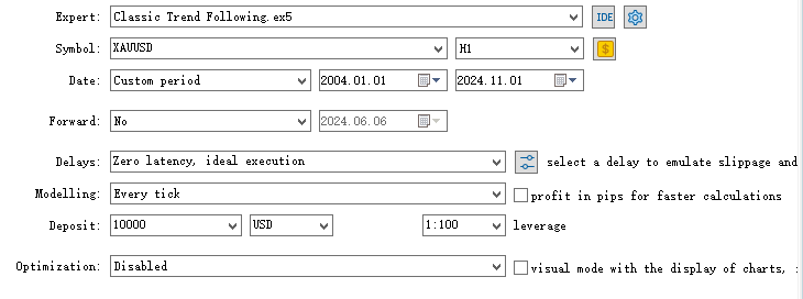
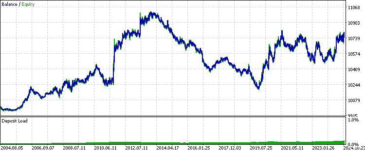
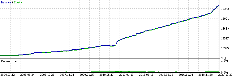
Finally, this is the test result on XAUUSD 1h timeframe, 2004.1.1 – 2024.11.1

Fetching Data
For training the model, we need the features values upon each trade, and we need to know the outcome of each trade. My most efficient and reliable way is to write an expert advisor that stores all the corresponding features into a 2-D array, and for the outcome data we simply export the trading report from the backtest.
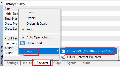
Firstly, to get the outcome data, we can simply go to the backtest and right click select report and open XML like this.
Next, to turn a double array into CSV, we'll use the CFileCSV class explained in this article.
We build on top of our backbone strategy script with the following steps:
1. Include the mqh file and create class object.
#include <FileCSV.mqh>

CFileCSV csvFile;
2. Declare the file name to be saved and the headers which have "index" and all the other feature names. The "index" here is merely used for updating the array index while running the tester and will get dropped later in python.
string fileName = "ML.csv";
string headers[] = {
    "Index",
    "Accelerator Oscillator",
    "Average Directional Movement Index",
    "Average Directional Movement Index by Welles Wilder",
    "Average True Range",
    "Bears Power",
    "Bulls Power",
    "Commodity Channel Index",
    "Chaikin Oscillator",
    "DeMarker",
    "Force Index",
    "Gator",
    "Market Facilitation Index",
    "Momentum",
    "Money Flow Index",
    "Moving Average of Oscillator",
    "MACD",
    "Relative Strength Index",
    "Relative Vigor Index",
    "Standard Deviation",
    "Stochastic Oscillator",
    "Williams' Percent Range",
    "Variable Index Dynamic Average",
    "Volume",
    "Hour",
    "Stationary"
};

string data[10000][26];
int indexx = 0;
vector xx;
3. We write a getData() function which calculates all the feature values and stores them into the global array. In this case, we use time, oscillators, and stationary price as features. This function will be called every time there's a trade signal so that it aligns with your trades. The selection of features will be mentioned later.
//+------------------------------------------------------------------+
//| Execute get data function                                        |
//+------------------------------------------------------------------+
vector getData(){
//23 oscillators
double ac[];        // Accelerator Oscillator
double adx[];       // Average Directional Movement Index
double wilder[];    // Average Directional Movement Index by Welles Wilder
double atr[];       // Average True Range
double bep[];       // Bears Power
double bup[];       // Bulls Power
double cci[];       // Commodity Channel Index
double ck[];        // Chaikin Oscillator
double dm[];        // DeMarker
double f[];         // Force Index
double g[];         // Gator
double bwmfi[];     // Market Facilitation Index
double m[];         // Momentum
double mfi[];       // Money Flow Index
double oma[];       // Moving Average of Oscillator
double macd[];      // Moving Averages Convergence/Divergence
double rsi[];       // Relative Strength Index
double rvi[];       // Relative Vigor Index
double std[];       // Standard Deviation
double sto[];       // Stochastic Oscillator
double wpr[];       // Williams' Percent Range
double vidya[];     // Variable Index Dynamic Average
double v[];         // Volume

CopyBuffer(handleAc, 0, 1, 1, ac);           // Accelerator Oscillator
CopyBuffer(handleAdx, 0, 1, 1, adx);         // Average Directional Movement Index
CopyBuffer(handleWilder, 0, 1, 1, wilder);   // Average Directional Movement Index by Welles Wilder
CopyBuffer(handleAtr, 0, 1, 1, atr);         // Average True Range
CopyBuffer(handleBep, 0, 1, 1, bep);         // Bears Power
CopyBuffer(handleBup, 0, 1, 1, bup);         // Bulls Power
CopyBuffer(handleCci, 0, 1, 1, cci);         // Commodity Channel Index
CopyBuffer(handleCk, 0, 1, 1, ck);           // Chaikin Oscillator
CopyBuffer(handleDm, 0, 1, 1, dm);           // DeMarker
CopyBuffer(handleF, 0, 1, 1, f);             // Force Index
CopyBuffer(handleG, 0, 1, 1, g);             // Gator
CopyBuffer(handleBwmfi, 0, 1, 1, bwmfi);     // Market Facilitation Index
CopyBuffer(handleM, 0, 1, 1, m);             // Momentum
CopyBuffer(handleMfi, 0, 1, 1, mfi);         // Money Flow Index
CopyBuffer(handleOma, 0, 1, 1, oma);         // Moving Average of Oscillator
CopyBuffer(handleMacd, 0, 1, 1, macd);       // Moving Averages Convergence/Divergence
CopyBuffer(handleRsi, 0, 1, 1, rsi);         // Relative Strength Index
CopyBuffer(handleRvi, 0, 1, 1, rvi);         // Relative Vigor Index
CopyBuffer(handleStd, 0, 1, 1, std);         // Standard Deviation
CopyBuffer(handleSto, 0, 1, 1, sto);         // Stochastic Oscillator
CopyBuffer(handleWpr, 0, 1, 1, wpr);         // Williams' Percent Range
CopyBuffer(handleVidya, 0, 1, 1, vidya);     // Variable Index Dynamic Average
CopyBuffer(handleV, 0, 1, 1, v);             // Volume
//2 means 2 decimal places
data[indexx][0] = IntegerToString(indexx);
data[indexx][1] = DoubleToString(ac[0], 2);       // Accelerator Oscillator
data[indexx][2] = DoubleToString(adx[0], 2);      // Average Directional Movement Index
data[indexx][3] = DoubleToString(wilder[0], 2);   // Average Directional Movement Index by Welles Wilder
data[indexx][4] = DoubleToString(atr[0], 2);      // Average True Range
data[indexx][5] = DoubleToString(bep[0], 2);      // Bears Power
data[indexx][6] = DoubleToString(bup[0], 2);      // Bulls Power
data[indexx][7] = DoubleToString(cci[0], 2);      // Commodity Channel Index
data[indexx][8] = DoubleToString(ck[0], 2);       // Chaikin Oscillator
data[indexx][9] = DoubleToString(dm[0], 2);       // DeMarker
data[indexx][10] = DoubleToString(f[0], 2);       // Force Index
data[indexx][11] = DoubleToString(g[0], 2);       // Gator
data[indexx][12] = DoubleToString(bwmfi[0], 2);   // Market Facilitation Index
data[indexx][13] = DoubleToString(m[0], 2);       // Momentum
data[indexx][14] = DoubleToString(mfi[0], 2);     // Money Flow Index
data[indexx][15] = DoubleToString(oma[0], 2);     // Moving Average of Oscillator
data[indexx][16] = DoubleToString(macd[0], 2);    // Moving Averages Convergence/Divergence
data[indexx][17] = DoubleToString(rsi[0], 2);     // Relative Strength Index
data[indexx][18] = DoubleToString(rvi[0], 2);     // Relative Vigor Index
data[indexx][19] = DoubleToString(std[0], 2);     // Standard Deviation
data[indexx][20] = DoubleToString(sto[0], 2);     // Stochastic Oscillator
data[indexx][21] = DoubleToString(wpr[0], 2);     // Williams' Percent Range
data[indexx][22] = DoubleToString(vidya[0], 2);   // Variable Index Dynamic Average
data[indexx][23] = DoubleToString(v[0], 2);       // Volume

    datetime currentTime = TimeTradeServer();
    MqlDateTime timeStruct;
    TimeToStruct(currentTime, timeStruct);
    int currentHour = timeStruct.hour;
data[indexx][24]= IntegerToString(currentHour);
    double close = iClose(_Symbol,PERIOD_CURRENT,1);
    double open = iOpen(_Symbol,PERIOD_CURRENT,1);
    double stationary = MathAbs((close-open)/close)*100;
data[indexx][25] = DoubleToString(stationary,2);

   vector features(26);
   for(int i = 1; i < 26; i++)
    {
      features[i] = StringToDouble(data[indexx][i]);
    }
    //A lot of the times positions may not open due to error, make sure you don't increase index blindly
    if(PositionsTotal()>0) indexx++;
    return features;
}
Note that we added a check here.
if(PositionsTotal()>0) indexx++;
This is because when your trade signal occurs, it may not result in a trade because the EA is running during market close time, but the tester won't take any trades.
4. We save the file upon OnDeInit() is called, which is when the test is over.
//+------------------------------------------------------------------+
//| Expert deinitialization function                                 |
//+------------------------------------------------------------------+
void OnDeinit(const int reason)
  {
   if (!SaveData) return;
   if(csvFile.Open(fileName, FILE_WRITE|FILE_ANSI))
     {
      //Write the header
      csvFile.WriteHeader(headers);
      //Write data rows
      csvFile.WriteLine(data);
      //Close the file
      csvFile.Close();
     }
   else
     {
      Print("File opening error!");
     }

  }
Run this expert advisor in the strategy tester, after that, you should be able to see your csv file formed in the /Tester/Agent-sth000 directory.
Cleaning and Adjusting Data
Now we have the two data files in the bag, but there remains many underlying problems to solve.
1. The backtest report is messy and is in .xlsx format. We only want whether we won or not for each trade.
First, we extract the rows where it only displays trade outcomes. You may need to scroll down your XLSX file until you see something like this:

Remember the row number and apply it to the following python code:
import pandas as pd

# Replace 'your_file.xlsx' with the path to your file
input_file = 'ML2.xlsx'

# Load the Excel file and skip the first {skiprows} rows
df = pd.read_excel(input_file, skiprows=10757)

# Save the extracted content to a CSV file
output_file = 'extracted_content.csv'
df.to_csv(output_file, index=False)

print(f"Content has been saved to {output_file}.")
Then we apply this extracted content to the following code to obtain the processed bin. Where winning trades would be 1 and losing trades would be 0.
import pandas as pd

# Load the CSV file
file_path = 'extracted_content.csv'  # Update with the correct file path if needed
data = pd.read_csv(file_path)

# Select the 'profit' column (assumed to be 'Unnamed: 10') and filter rows as per your instructions
profit_data = data["Profit"][1:-1]
profit_data = profit_data[profit_data.index % 2 == 0]  # Filter for rows with odd indices
profit_data = profit_data.reset_index(drop=True)  # Reset index
# Convert to float, then apply the condition to set values to 1 if > 0, otherwise to 0
profit_data = pd.to_numeric(profit_data, errors='coerce').fillna(0)  # Convert to float, replacing NaN with 0
profit_data = profit_data.apply(lambda x: 1 if x > 0 else 0)  # Apply condition

# Save the processed data to a new CSV file with index
output_csv_path = 'processed_bin.csv'
profit_data.to_csv(output_csv_path, index=True, header=['bin'])

print(f"Processed data saved to {output_csv_path}")
The result file should look something like this
| bin | |
|---|---|
| 0 | 1 |
| 1 | 0 |
| 2 | 1 |
| 3 | 0 |
| 4 | 0 |
| 5 | 1 |
Note that if all the values are 0 it may be because your starting rows are incorrect, make sure to check whether your starting row is now even or odd and change it accordingly with the python code.
2. The feature data is all string due to the CFileCSV class, and they're stuck together in one column, only separated by commas.
The following python code gets the job done.
import pandas as pd

# Load the CSV file with semicolon separator
file_path = 'ML.csv'
data = pd.read_csv(file_path, sep=';')

# Drop rows with any missing or incomplete values
data.dropna(inplace=True)

# Drop any duplicate rows if present
data.drop_duplicates(inplace=True)

# Convert non-numeric columns to numerical format
for col in data.columns:
    if data[col].dtype == 'object':
        # Convert categorical to numerical using label encoding
        data[col] = data[col].astype('category').cat.codes

# Ensure all remaining columns are numeric and cleanly formatted for CatBoost
data = data.apply(pd.to_numeric, errors='coerce')
data.dropna(inplace=True)  # Drop any rows that might still contain NaNs after conversion

# Save the cleaned data to a new file in CatBoost-friendly format
output_file_path = 'Cleaned.csv'
data.to_csv(output_file_path, index=False)

print(f"Data cleaned and saved to {output_file_path}")
Finally, we use this code to merge the two files together so that we can easily access them as a single data frame in the future.
import pandas as pd

# Load the two CSV files
file1_path = 'processed_bin.csv'  # Update with the correct file path if needed
file2_path = 'Cleaned.csv'  # Update with the correct file path if needed
data1 = pd.read_csv(file1_path, index_col=0)  # Load first file with index
data2 = pd.read_csv(file2_path, index_col=0)  # Load second file with index

# Merge the two DataFrames on the index
merged_data = pd.merge(data1, data2, left_index=True, right_index=True, how='inner')

# Save the merged data to a new CSV file
output_csv_path = 'merged_data.csv'
merged_data.to_csv(output_csv_path)

print(f"Merged data saved to {output_csv_path}")
To confirm that two data is correctly merged, we can check the three CSV files we just produced and see if their final index is the same. If so, we're most likely chillin'.
Training Model
We won't go too in depth into the technical explanations behind each aspect of machine learning. However, I strongly encourage you to check out Advances in Financial Machine Learning by Marcos López de Prado if you're interested in ML trading as a whole.
Our objective for this section is crystal clear.
First, we use the pandas library to read the merged data and split the bin column as y and the rest as X.
data = pd.read_csv("merged_data.csv",index_col=0)
XX = data.drop(columns=['bin'])
yy = data['bin']
y = yy.values
X = XX.values
Then we split the data into 80% for training and 20% for testing.
We then train. The details of each parameter in the classifier are documented on the CatBoost website.
from catboost import CatBoostClassifier
from sklearn.ensemble import BaggingClassifier

# Define the CatBoost model with initial parameters
catboost_clf = CatBoostClassifier(
    class_weights=[10, 1],  #more weights to 1 class cuz there's less correct cases
    iterations=20000,             # Number of trees (similar to n_estimators)
    learning_rate=0.02,          # Learning rate
    depth=5,                    # Depth of each tree
    l2_leaf_reg=5,
    bagging_temperature=1,
    early_stopping_rounds=50,
    loss_function='Logloss',    # Use 'MultiClass' if it's a multi-class problem
    random_seed=RANDOM_STATE,
    verbose=1000,                  # Suppress output (set to a positive number if you want to see training progress)
)

fit = catboost_clf.fit(X_train, y_train)
We save the .cbm file.
catboost_clf.save_model('catboost_test.cbm') Unfortunately, we're not done yet. MetaTrader 5 only supports ONNX format model, so we use the following code from this article to transform it into ONNX format.
model_onnx = convert_sklearn(
    model,
    "catboost",
    [("input", FloatTensorType([None, X.shape[1]]))],
    target_opset={"": 12, "ai.onnx.ml": 2},
)

# And save.
with open("CatBoost_test.onnx", "wb") as f:
    f.write(model_onnx.SerializeToString())
Statistical Testing
After obtaining the .onnx file, we drag it into the MQL5/Files folder. We now build on top of the expert advisor we used to fetch data earlier. Again this article already explains the procedure of initializing .onnx model in expert advisors in detail, I would just emphasize on how we change the entry criteria.
     if (maFast[1]>maSlow[1]&&maFast[0]<maSlow[0]&&sellpos == buypos){
        xx= getData();
        prob = cat_boost.predict_proba(xx);
        if (prob[1]<max&&prob[1]>min)executeBuy();
     }
     if(maFast[1]<maSlow[1]&&maFast[0]>maSlow[0]&&sellpos == buypos){
        xx= getData();
        prob = cat_boost.predict_proba(xx);
        Print(prob);
        if(prob[1]<max&&prob[1]>min)executeSell();
      }
Here we call getData() to store the vector information in variable xx, then we return the probability of success according to the model. We added a print statement so that we get a sense of what range it's going to be. For trend-following strategy, because of its low accuracy and high reward-to-risk ratio per trade, we normally see the model give probability less than 0.5.
We add a threshold for filtering out trades that display low probability of success, and we have finished the coding part. Now let's test.
Remember we split it to 8-2 ratio? Now we're going to do an out-of-sample test on the untrained data, which is approximately 2021.1.1-2024.11.1.
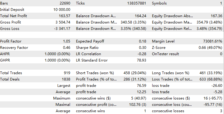
We first run the in-sample test with a 0.05 probability threshold to confirm we trained with the right data. The result should be almost perfect like this.
Then we run an out-of-sample test with no threshold as baseline. We expect, if we scale up the threshold, we should beat this baseline result by quite a margin.

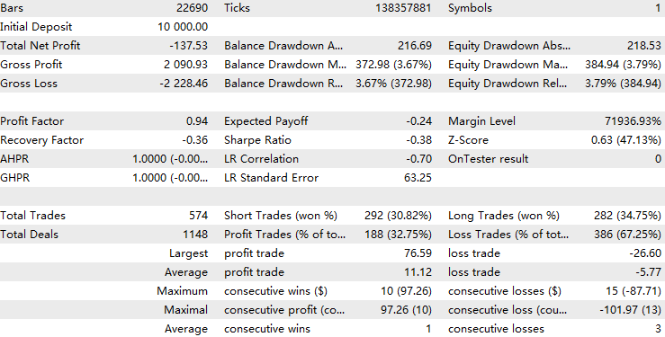
Finally, we conduct out-of-sample tests to analyze the profitability patterns relative to different thresholds.
Results of threshold = 0.05:

Results of threshold = 0.1:

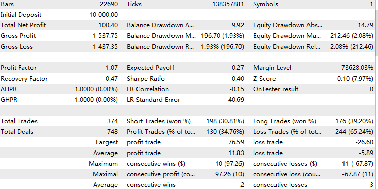
Results of threshold = 0.2:

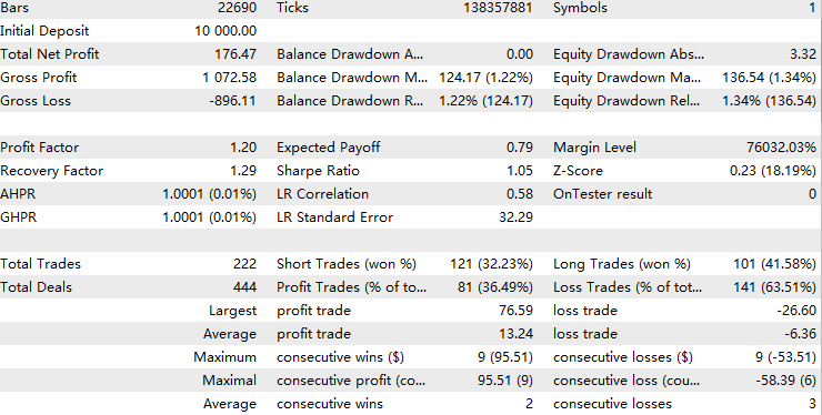
For a threshold of 0.05, the model filtered out approximately half of the original trades, but this led to a decrease in profitability. This could suggest that the predictor is overfitted, becoming too attuned to the trained patterns and failing to capture the similar patterns shared between the training and testing sets. In financial machine learning, this is a common issue. However, when the threshold is increased to 0.1, the profit factor gradually improves, surpassing that of our baseline.
At a threshold of 0.2, the model filters out about 70% of the original trades, but the overall quality of the remaining trades is significantly more profitable than the original ones. Statistical analysis shows that within this threshold range, overall profitability is positively correlated with the threshold value. This suggests that as the model's confidence in a trade increases, so does its overall performance, which is a favorable outcome.
I ran a ten-fold cross validation in python to confirm that the model precision is consistent.
{'score': array([-0.97148655, -1.25263677, -1.02043177, -1.06770248, -0.97339545, -0.88611439, -0.83877111, -0.95682533, -1.02443847, -1.1385681 ])} The difference between each cross-validation score is mild, indicating that the model's accuracy remains consistent across different training and testing periods.
Additionally, with an average log-loss score around -1, the model's performance can be considered moderately effective.
To further improve the model precision, one may pick up on the following ideas:
1. Feature engineering
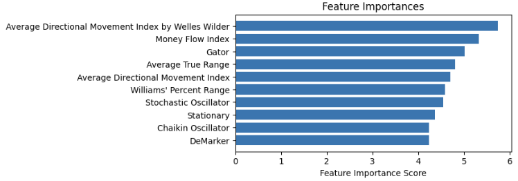
We plot the feature importance like this and remove the ones that have little importance.
For selecting features, anything market related is plausible, but make sure you make the data stationary because tree-based models use fixed value rules to process inputs.
2. Hyperparameter tuning
Remember the parameters in the classifier function I talked about earlier? We could write a function to loop through a grid of values and test which training parameter would yield the best cross validation scores.
3. Model selection
We can try different machine learning models or different types of values to predict. People have found that while machine learning models are bad at predicting prices, it is rather competent in predicting volatility. Besides, hidden Markov model is widely used to predict hidden trends. Both of these could be potent filters for trend following strategies.
I encourage the readers to try these methods out with my attached code, and let me know if you found any success in improving the performance.
Conclusion
In this article, we walked through the entire workflow of developing a CatBoost machine learning filter for a trend-following strategy. On the way, we highlighted different aspects to be aware of while researching machine learning strategies. In the end, we validated the strategy through statistical testing and discussed future aspirations extending from the current approach.
Attached File Table
| File name | Usage |
|---|---|
| ML-Momentum Data.mq5 | The EA to fetch features data |
| ML-Momentum.mq5 | Final execution EA |
| CB2.ipynb | The workflow to train and test CatBoost model |
| handleMql5DealReport.py | extract useful rows from deal report |
| getBinFromMql5.py | get binary outcome from the extracted content |
| clean_mql5_csv.py | Clean the features CSV extracted from Mt5 |
| merge_data2.py | merge features and outcome into one CSV |
| OnnxConvert.ipynb | Convert .cbm model to .onnx format |
| Classic Trend Following.mq5 | The backbone strategy expert advisor |
 MQL5 Trading Toolkit (Part 4): Developing a History Management EX5 Library
 Trading with the MQL5 Economic Calendar (Part 5): Enhancing the Dashboard with Responsive Controls and Filter Buttons
 Creating a Trading Administrator Panel in MQL5 (Part VIII): Analytics Panel
 Reimagining Classic Strategies (Part 12): EURUSD Breakout Strategy
- Free trading apps
- Over 8,000 signals for copying
- Economic news for exploring financial markets
You agree to website policy and terms of use
Your point is absolutely valid. In my experience, I also find that using recent data makes it easier to train a model that produces better results. However, the main issue is that this approach limits the size of the training set unless you use a very short timeframe. Trend-following strategies perform better over longer timeframes compared to shorter ones according to academic papers. So you might train a model with higher predictability but fewer training samples, which is prone to overfitting, and the original strategy has less edge to begin with. There is a tradeoff between these factors, not to mention that spreads also play a role.
My solution to this is to assign greater weights to recent data in the training set while still preserving older data. In this way, we can adapt to new patterns after a regime shift while still benefiting from old patterns that have stayed consistent over the years. However, as I mentioned earlier, there are always trade-offs involved in these decisions.
Retraining the model every three months using the latest three months of data would probably do the trick. I’ll try to implement this rolling model optimization idea later. Thanks for the suggestion.
I am trying to follow your instructions and sadly due to a lack of detail am not able to continue through to the final output due to missing file references and no download links
I will take the time to teach you what you have missed because this looks like a good process.
You are missing;
1. A direct link to FileCSV.mqh which requires going through the other article to obtain it.
2. declaration of all of the features handles
3. Adequate explanation of the process for either creating or downloading the files
CatOnnx.mqh
"\\Files\\CatBoost_Momentum_test.onnx"
4. Direct links to and relevant instructions on how to install catboot using pip or similar making sure you have the dependencies installed that are required for python. (not for me but others will need to know)
5. Instruction to read the CB2.ipynb instructions and workflow.
Overall this all leads to the student getting half way through your article and being left searching for hours for the correct process to complete the tutorial and replicate your results.
Overall I give this article a 4 out of 10 for information with additional points for your Classic Trend Following Strategy which is well put together.
Please edit the article to be more instructive and step by step so we can all learn and follow.
PS
recommendations on how this could be adapted to other strategies would be great!
Thanks for the feedback. Unfortunately I ended up only briefly describing the relevant articles because I thought it would take up too much space, and I didn't include download links due to copyright issues. The thorough details would still be best obtained from the original source. Nevertheless, I do think I overlooked some careful instructions for my python code and direct links to python instructions although I added comments for each line. If you have specific obstacles in your own implementation process, you can discuss here or add me to chat.
The CatOnnx.mqh called in the ML-Momentum.mq5 file is the same as the CatBoost.mqh as I cited in this article. Sorry for causing confusions in the file names.
Thanks great to get some clarification this looks very interesting, when I go back and try again to complete the guide in this article I will keep some notes aside for later forum fertilization.
If anyone else is interested in cat farming...