Robustness Testing on Expert Advisors

Introduction

In strategy development, there are many intricate details to consider, many of which are not highlighted for beginner traders. As a result, many traders, myself included, have had to learn these lessons the hard way. This article is based on my observations of common pitfalls that most beginner traders encounter when developing strategies on MQL5. It will offer a range of tips, tricks, and examples to help identify the disqualification of an EA and test the robustness of our own EAs in an easy-to-implement way. The goal is to educate readers, helping them avoid future scams when purchasing EAs as well as preventing mistakes in their own strategy development.

Red Flags on the EA Market

A quick glance at the MQL5 market reveals that it is dominated by sellers promoting AI trading systems using popular large language models like ChatGPT or Gemini AI. I firmly believe that none of these claims are genuine for one simple reason: it is impossible to use commercial LLMs for backtesting without introducing look-ahead bias. Furthermore, the integration of popular LLMs with MQL5 uses the web requesting function. So if a seller doesn't specify that the EA require internet or prompting, it's unlikely to be legitimate. A more robust approach to incorporating LLMs in trading would involve live testing or building on top of primitive models like BERT. A recent paper exemplifies this approach.

However, there is something to clarify here. AI doesn't only mean large language models, though most people assume it is. Most of the advanced machine learning techniques, including unsupervised learning, supervised learning, and reinforcement learning, can be classified as using AI for their EAs. So it isn't false marketing if a seller claims to sell an AI EA when they're using some neural network models. Unfortunately, most of the AI EAs don't use even basic neural network models, despite claiming to do so. One way to verify this is by checking whether they provide an additional ONNX file. If the product consists only of an executable file, they must have hardcoded all the model parameters into the EA, which usually results in a file size of over a megabyte.

Some other red flags in the EA market include:

• Very large stop losses compared to take profits. Often, they use indicators to filter out losing trades in backtest, making losses rare and creating the illusion of a high win rate. In reality, a single loss can wipe out numerous profitable trades.
• The seller only invests a small amount in their signal, such as $10-$100, while selling the EA for $1,000 or more. This suggests they anticipate the account will eventually blow up and are attempting to capitalize on the high percentage gains from a small account.
• The account is new, with only a few trades, creating a 100% win rate in the signal.
• Use of Martingale, hedging, dollar-cost averaging, or grid systems. These strategies increase risk by multiplying positions after a loss or adding more trades in the same direction during a drawdown. These classic approach date back to the 20th century, and are unlikely to be the "hidden holy grail" strategies because their expected returns are less than or equal to zero.

Here's a brief mathematical proof:

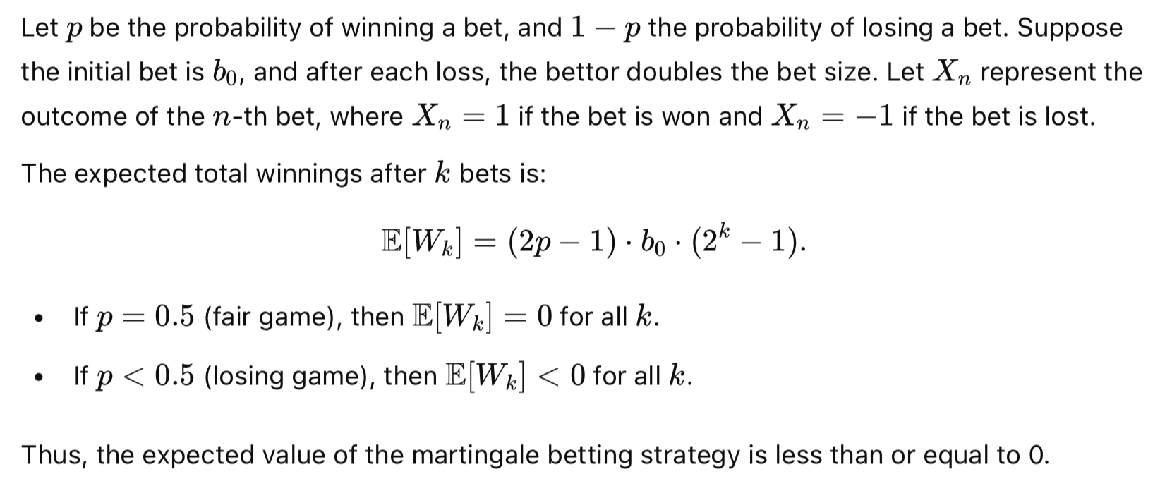
If their backbone strategies don't have a clear edge already (p significantly larger than 0.5), the expectation of return is less than or equal to zero, meaning you'll be losing in the long run and the loss just hasn't been realized yet. Even if a martingale or grid system is built on top of a profitable entry, you're ultimately still risking your entire portfolio balance each trade, not a fraction like most risk management approaches. If you're uncertain that you will be able to keep depositing more money when the account is in huge drawdown, then I'll advise you not to use them.

One thing to clarify is that this section aims to raise awareness of common false marketing techniques prevalent in today’s MQL5 market, and is not a protest against selling or buying EAs on MQL5. In fact, I encourage more people to sell EAs on MQL5, based on trustworthy marketing and genuinely robust EAs, to help make it a more credible environment.

Overfitting

Overfitting is a common issue in trading models, where a strategy might perform well on historical data but fail to generalize to new, unseen data. In this experiment, we will use a python code to demonstrate how overfitting can occur due to the selection of parameters in a trading model. Specifically, we will generate random trading scenarios with multiple features, visualize the impact of selective filtering, and observe how performance varies when parameters are overly optimized for a specific subset of the data.

We start by simulating a dataset of 1000 random trading samples, where each sample corresponds to a trading decision with three features:

• Feature 1: This could represent various market conditions, such as 'a', 'b', or 'c'.
• Feature 2: Represents another factor like 'd', 'e', or 'f', such as asset volatility or sentiment.
• Feature 3: This might represent other trading indicators, with values like 'g', 'h', or 'i'.

import numpy as np
import pandas as pd
import seaborn as sns
import matplotlib.pyplot as plt

# Step 1: Generate random samples
np.random.seed(42)  # For reproducibility

# Possible feature values
feature_1_values = ['a', 'b', 'c']
feature_2_values = ['d', 'e', 'f']
feature_3_values = ['g', 'h', 'i']

# Generate random data
n_samples = 1000
feature_1 = np.random.choice(feature_1_values, n_samples)
feature_2 = np.random.choice(feature_2_values, n_samples)
feature_3 = np.random.choice(feature_3_values, n_samples)
outcome = np.random.choice([0, 1], n_samples)  # Random binary outcome

# Create a DataFrame
df = pd.DataFrame({
    'feature_1': feature_1,
    'feature_2': feature_2,
    'feature_3': feature_3,
    'outcome': outcome
})

Each of these samples will have an associated outcome (either a win or a loss), randomly assigned as either 0 or 1. These outcomes represent the result of a hypothetical trade based on the given features, which denotes different parameter values.

In real-world trading, selecting the right parameters (such as market indicators, trading time windows, or thresholds for buy/sell signals) is crucial for model performance. However, overfitting occurs when the model is excessively tuned to fit specific patterns in historical data that do not generalize well to new data.

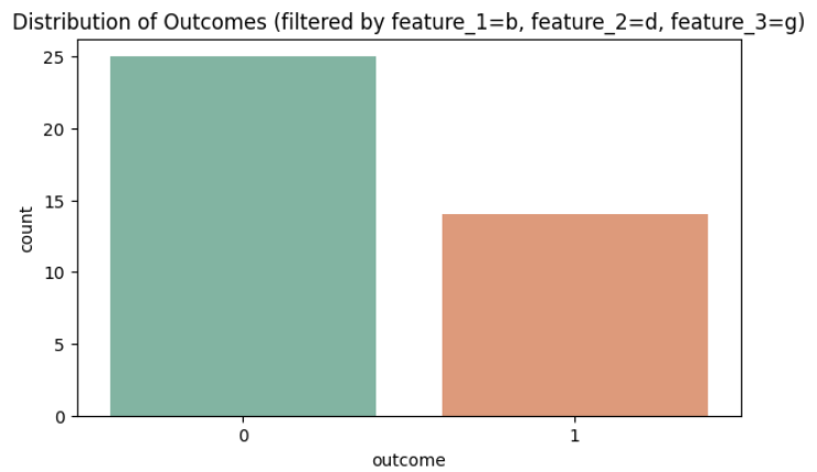
To demonstrate this, we first only consider samples where Feature 1 = 'b', Feature 2 = 'd', and Feature 3 = 'g'.

def plot_filtered_distribution(df, feature_filters):
    # Filter the DataFrame based on the specified feature values
    filtered_df = df
    for feature, value in feature_filters.items():
        filtered_df = filtered_df[filtered_df[feature] == value]
    
    # Check if filtered dataframe is empty
    if filtered_df.empty:
        print("No data available for the selected feature combination.")
        return

    # Plot the distribution of outcomes based on the filtered data
    sns.countplot(x='outcome', data=filtered_df, palette='Set2')
    plt.title(f'Distribution of Outcomes (filtered by {", ".join([f"{key}={value}" for key, value in feature_filters.items()])})')
    plt.show()

# Example usage: Visualize the distribution of outcomes when filtering by feature_1 = 'a', feature_2 = 'd', feature_3 = 'g'
plot_filtered_distribution(df, {'feature_1': 'b', 'feature_2': 'd', 'feature_3': 'g'})

Then we plot the outcome distribution considering samples where Feature 1 = 'c', Feature 2 = 'f', and Feature 3 = 'h'.

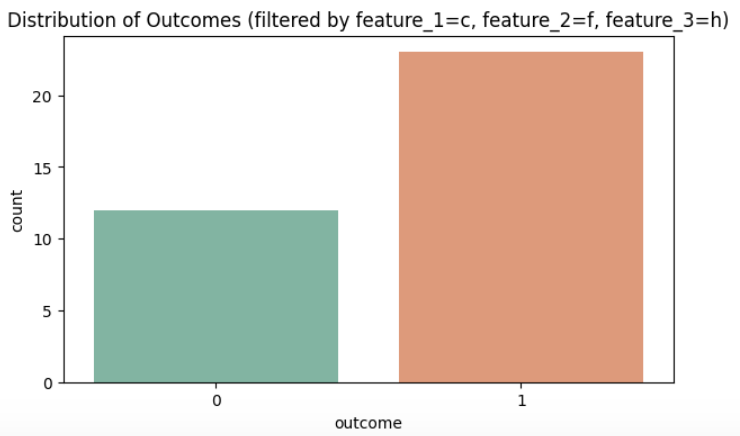
We can clearly see that by only changing three parameters in this randomly generated data, we're able to pick out a set that is mostly dominated by losses or by wins. This goes to show the power of overfitting. By focusing on a specific subset of features, we force the model to fit to a narrow slice of the data, which can lead to misleading conclusions. The more selectively we filter the data based on the features, the more likely we are to observe an artificially high performance (in terms of outcomes), which is a hallmark of overfitting. Any arbitrary strategy, with enough parameters to overfit, it will inevitably be able to yield results that are profitable.

This is a critical warning for traders who rely on finely tuned strategies based on specific parameter sets, as they may not generalize well to future market conditions. The key takeaway is that model robustness—where performance is consistent across a broad range of data—is far more valuable than optimizing for narrow parameter ranges.

Optimization on MetaTrader 5 Terminal

When we attempt to select the optimal values for a specific EA's performance over a given period, we are engaging in optimization. As demonstrated in the previous section, it is easy to overfit a small sample of random data by making small adjustments to a few parameters. This raises the question: how can we avoid this mistake in optimization and make our backtest results more credible? This section will explore several ways to minimize the risk of overfitting and ensure more robust results when performing optimization on the MetaTrader 5 terminal.

1. More Samples Over a Longer Period

According to the law of large numbers, assuming the returns of your strategy follow some form of distribution, the mean return of your samples will approximate the mean of that distribution as the number of samples increases. For strategies that are not as high-frequency as day trading or scalping, it is recommended to test them with data spanning at least 10 years and including thousands of trades. If your strategy is sensitive to macro regime shifts, testing only on recent years is acceptable. However, ultimately, you need enough samples to validate the strategy, as there is no universal rule for how many samples are enough. The goal is to demonstrate that a historical, repeating pattern exists that can be exploited in the financial markets. 

If your EA operates on a higher timeframe, you can test it across multiple assets to gather more samples, potentially transforming it into a multi-asset strategy. This approach significantly reduces the likelihood of overfitting, as the strategy’s performance will be tested across a broader range of market conditions and asset behaviors. By diversifying the assets tested, you increase the robustness of your strategy and enhance its ability to adapt to different market environments.

2. Fewer Tunable Parameters

As shown in the previous experiment, the more parameters you have, the more ways the optimization process can filter out groups of winning samples. A parameter that is randomly generated at the beginning can easily be filtered into a group of successful results, but this does not necessarily prove the validity of the entire sample set. David Aronson, in Evidence-Based Technical Analysis, investigated the use of data-mining techniques and concluded that a single tunable parameter strategy is unlikely to exist, although it would be less prone to overfitting. The recommended approach is to keep the number of tunable parameters to fewer than five. Parameters that do not affect the results, such as magic numbers, should not be considered tunable. Parameters like the look-back period of indicators can be fixed to widely accepted values, and in such cases, they should not be counted as tunable parameters during optimization.

3. Account for Commissions, Spreads, and Swaps in Your Backtest and Optimization

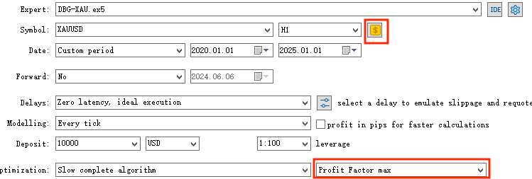
When using the strategy tester, be sure to click on the money sign and check if commissions, spreads, and swaps are set to reflect the conditions of your live trading environment. 

Many traders mistakenly believe that if their strategy is consistently losing, it means they are doing the opposite of what a winning strategy would do. They may think that by simply flipping their trading direction, they will consistently win. However, this is far from the truth. Trading is a negative-sum game for retail traders. A consistently losing trader is more likely to have a strategy that no longer has an edge, and their results follow a random distribution of wins and losses. In such cases, the losses are often due to the spreads, commissions, and swap fees paid with each trade.

It is far less likely that you could develop a strategy that consistently produces the opposite signals of a profitable strategy, compared to creating a profitable strategy yourself. In the latter case, you're actively working to make the strategy win, while in the former, you're not.

This is why I don’t recommend beginner traders try scalping strategies— the relative statistical disadvantage is simply too great. Let’s consider an example: If you're trading EUR/USD, the typical conditions for a b-book broker are no commissions but a 1-pip spread, and for an ECN a-book broker, the conditions are a $7 commission per lot with a 0.1-pip spread. If you're attempting to scalp only a 10-pip take-profit, in either case, you're effectively paying around a 10% commission on each trade, whether you win or lose. This is particularly problematic for high-frequency traders, as those costs will gradually erode profits over time.

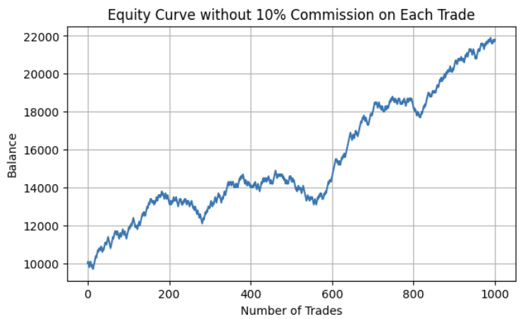
Now, suppose you have a robust strategy with a 55% win rate and a 1:1 risk-to-reward ratio. Without factoring in spreads or commissions, your equity curve would look pretty nice even by professional standard:

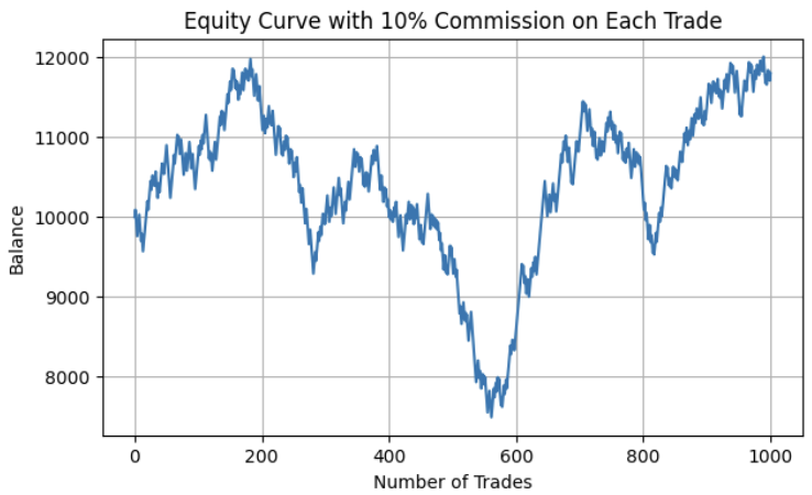
But if you factor in that 10% cost from the commissions, spreads, and swaps due to your attempt to scalp small trades, effectively increasing the relative cost of each trade, your equity curve would become barely profitable, as shown below:

Simulation python code:

import numpy as np
import matplotlib.pyplot as plt
import pandas as pd

# Parameters
n_trades = 1000  # Number of trades
win_rate = 0.55  # 55% win rate
commission_rate = 0.1  # 10% commission per trade
initial_balance = 10000  # Starting balance
trade_amount = 100  # Amount per trade

# Simulate the trades
np.random.seed(42)  # For reproducibility

# Generate random outcomes (1 for win, 0 for loss)
outcomes = np.random.choice([1, 0], size=n_trades, p=[win_rate, 1 - win_rate])

# Initialize balance and equity curve
balance = initial_balance
equity_curve = [balance]

# Simulate each trade
for outcome in outcomes:
    # Calculate the result of the trade
    if outcome == 1:
        # Win: add profit (trade_amount) and subtract commission
        balance += trade_amount - (trade_amount * commission_rate)
    else:
        # Loss: subtract loss (trade_amount) and subtract commission
        balance -= trade_amount + (trade_amount * commission_rate)
    
    # Append the updated balance to the equity curve
    equity_curve.append(balance)

# Plot the equity curve
plt.figure(figsize=(7, 4))
plt.plot(equity_curve)
plt.title('Equity Curve with 10% Commission on Each Trade')
plt.xlabel('Number of Trades')
plt.ylabel('Balance')
plt.grid(True)
plt.show()

4. Take Bigger Steps in the Optimization Process and Mind the Parameter Sensitivity

In the MetaTrader 5 optimization terminal, you can adjust the step size for each parameter trial. It's recommended to use larger steps relative to the usual value of the parameter. Focusing on very specific values can easily lead to overfitting and sensitivity to regime shifts. For example, last year, a mean-reversion strategy might have worked best with an RSI look-back period of 11, but this year it could be 13. If we focus on small, incremental values, we may miss the broader performance patterns relative to the parameters and waste time on inefficient optimization.

Personally, I prefer using profit factor as a metric to indicate performance, as it’s a ratio rather than an absolute number like total return.

Profit factor = Gross Profit / Gross Loss.

Parameter sensitivity is also crucial. We want to ensure that our trials cover a broad range of possible values for each parameter. Ideally, the area around the best value should show a concave distribution, where performance gradually decreases at a steady rate as the parameter value deviates from the optimal setting. This ensures that the strategy maintains its edge despite variations in parameter values, and that the best performance parameters represent the optimal setting for the strategy.

Out-of-sample Testing

Whether you're optimizing parameters or testing the EA on different timeframes and symbols, it's best to exclude recent data from your tests. These data points should be outside your knowledge domain before making any changes to your original EA. This approach is known as in-sample/out-of-sample testing.

The goal of this testing method is to avoid look-ahead bias, where changes to your EA are based on known characteristics of recent market behavior. It also helps reduce the risk of overfitting during optimization.

To implement this, first decide on the total sample size you plan to test. Based on the number of sample tests, you can choose an in-sample to out-of-sample ratio, such as 7:3, 8:2, or 9:1. You then make all observations, assumptions, and changes to parameter values and signal rules using the in-sample data. Afterward, apply the final EA to backtest on the out-of-sample data to check if your assumptions hold consistently. If an EA that was optimized to yield excellent results in the in-sample test becomes barely profitable or even loses in the out-of-sample test, this could suggest either edge erosion due to recent regime shifts or overfitting during in-sample optimization.

When evaluating whether the consistency of an EA holds through in-sample and out-of-sample testing, there are several key metrics to consider.

Firstly, you should create a version of your EA without the leverage compounding effect, as this could distort the results and place undue importance on the tail of the sample set.

Here are the main metrics to look for:

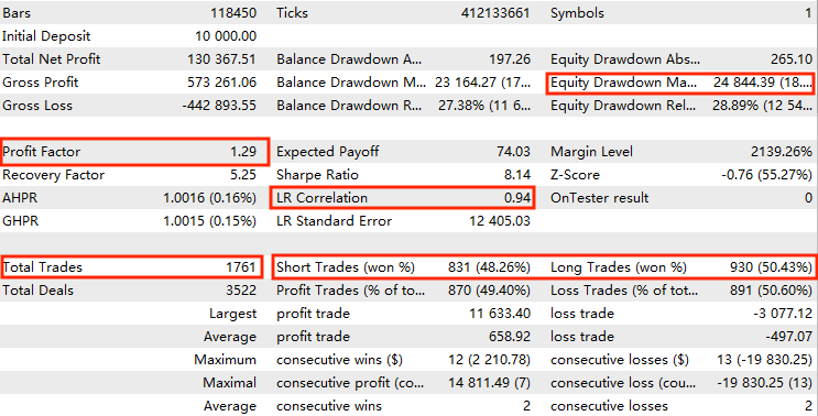
1. Profit Factor: The profit factor should be greater than 1, with a reasonable range between 1.2 and 1.5. A profit factor lower than 1.2 may indicate that the strategy is not profitable enough, while a value higher than 1.5 could suggest that the sample size is too small or that trading costs were not accounted for. While this doesn't necessarily mean your strategy is fraudulent, you should be cautious if the results seem unrealistic.

2. Maximum Equity Drawdown: Focus on the maximum equity drawdown rather than the absolute drawdown, as it reflects the potential risk rather than the risk that has already occurred. The maximum equity drawdown should be at least 10% lower than your personal maximum drawdown tolerance. If it's too low, you can consider increasing your EA’s risk, and if it's too high, you may need to reassess the risk profile of your strategy.

3. LR Correlation: The linear regression (LR) correlation measures the consistency of your equity curve. A correlation of greater than 0.9 signals that the returns were relatively consistent throughout the testing period. This helps ensure that the strategy doesn't have large fluctuations and that the performance is steady.

4. Win Rate and Trade Volume for Long and Short Positions: If your EA trades both long and short positions, ensure that their win rates and trade volumes are reasonably similar. A significant discrepancy between the two could signal an imbalance in the strategy that may need to be addressed.

While other metrics are also important, these three are the primary factors to be aware of when assessing the reliability of your EA during in-sample and out-of-sample testing.

Some traditional traders prefer walk-forward analysis, where the in-sample/out-of-sample test is performed piece by piece, "walking forward" until the current time. However, I believe that this is often unnecessary, especially if we've already ensured that our parameters are few in number and not overfitted to overly specific values. In such cases, it's very likely that these optimal parameter values will remain consistent over time. Furthermore, we’ve already emphasized that the key to a strategy's edge lies in its signal rules, not its parameter values. Therefore, a single in-sample/out-of-sample test is typically sufficient to validate the results.

That said, for machine learning-based strategies, the situation is different. The edge in these strategies often comes from the underlying machine learning model's parameters, which may vary significantly depending on the time period of the training data. In this case, walk-forward analysis becomes necessary to account for how model performance might change with different data sets over time. I have provided a detailed explanation of how to implement walk-forward analysis in this article. Ultimately, the key takeaway is that the EA must remain somewhat profitable in recent times to confirm its continued viability.

Outliers Testing

Outlier testing ensures that your profits are not driven by a few outlier trades that account for most of the gains, but rather stem from consistent, balanced gains and losses. This is important because if profits are primarily due to a few outliers, it undermines the value of having more samples to approximate the mean return. To check for this, simply examine your backtest equity curve and ensure that its upward movement is not caused by a few large spikes but rather by steady, consistent growth. Additionally, you can confirm this by comparing the largest gain to the average gain in the backtest report.

We also want to ensure that profits are not primarily concentrated in a short period of time, as this could indicate temporary regime bias. To check for this, we examine the distribution of monthly returns to ensure consistency. First, obtain the backtest report by right-clicking on the report and saving it. 

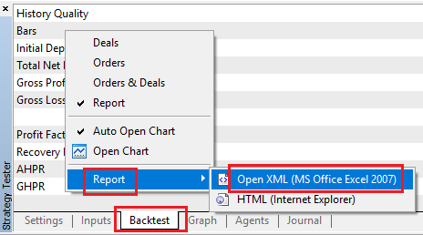
Then, open the file and note the row number of the "Deals" row (in this example, it’s 9342).

Finally, you can use Python in Jupyter Notebook to run the following code to output a table of monthly returns in percentage.

import pandas as pd
import matplotlib.pyplot as plt
# Replace 'your_file.xlsx' with the path to your file
input_file = 'your_backtest.xlsx'
# Load the Excel file and skip the first {skiprows} rows, skiprows = the row of "DEAL"
data = pd.read_excel(input_file, skiprows=9342)
# Select the 'profit' column (assumed to be 'Unnamed: 10') and filter rows as per your instructions
profit_data = data[['Time','Symbol','Profit','Balance']][1:-1] 
profit_data = profit_data[profit_data.index % 2 == 0]  # Filter for rows with odd indices
profit_data = profit_data.reset_index(drop=True)  # Reset index
# Convert to float, then apply the condition to set values to 1 if > 0, otherwise to 0
profit_data[['Profit','Balance']] = profit_data[['Profit','Balance']].apply(pd.to_numeric, errors='coerce').fillna(0)  # Convert to float, replacing NaN with 0

# Load the data
data = profit_data

# Calculate percentage gain compared to the previous balance
data['percentage_gain'] = data['Profit'] / data['Balance'].shift(1) * 100

# Drop the first row because it doesn't have a previous balance to compare
data = data.dropna()

# Ensure 'time' is in datetime format
data['Time'] = pd.to_datetime(data['Time'])

# Extract the year and month from the 'time' column
data['year'] = data['Time'].dt.year
data['month'] = data['Time'].dt.month_name()

# Ensure months are ordered correctly (January to December)
month_order = ['January', 'February', 'March', 'April', 'May', 'June', 'July', 'August', 'September', 'October', 'November', 'December']
data['month'] = pd.Categorical(data['month'], categories=month_order, ordered=True)

# Calculate the total return for each year-month combination
monthly_return = data.groupby(['year', 'month'])['percentage_gain'].sum().unstack(fill_value=0)

# Function to apply color formatting based on return value
def colorize(val):
    color = 'green' if val > 0 else 'red'
    return f'background-color: {color}'

# Display the table with color coding
styled_table = monthly_return.style.applymap(colorize, subset=pd.IndexSlice[:, :])

# Show the table
styled_table

Drawdown months are almost inevitable in long-term backtests, but here we need to focus on the return percentage and confirm that none of the drawdowns are significantly larger than the mean return of the entire sample set.

Lastly, if your EA trades multiple assets, we must ensure that no single asset is responsible for the majority of the profits, while others contribute little. To do this, we can extend our original Python code by adding lines to generate a pie chart showing the return distribution across different assets.

import seaborn as sns
# Group by symbol and calculate the total profit/loss for each symbol
symbol_return = data.groupby('Symbol')['percentage_gain'].sum()

# Plot the pie chart
plt.figure(figsize=(7, 3))
plt.pie(symbol_return, labels=symbol_return.index, autopct='%1.1f%%', startangle=90, colors=sns.color_palette("Set2", len(symbol_return)))

# Title and display
plt.title('Total Return by Symbol')
plt.show()

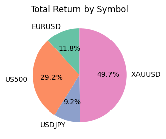
We simply need to ensure that no single asset dominates the pie chart.

Advanced Suggestions

Here I list out four more advanced robustness tests that may require more expertise and time.

1. Live Trading Testing: 

Implement the strategy in a real or paper trading environment with small position sizes, and monitor its performance over time in real market conditions. Live trading tests the strategy’s ability to handle real market dynamics, including slippage, spreads, and execution delays.

It helps assess if the strategy can perform as expected under real trading conditions and emotional pressure, beyond backtesting or simulations.

2. Monte Carlo Simulation: 

Run a Monte Carlo simulation by randomly shuffling the order of trade outcomes (wins and losses) and generating a large number of possible equity curves. This can also include random adjustments to parameters like entry points or stop losses.

Monte Carlo simulations help evaluate how robust a strategy is to random market conditions, offering insight into potential worst-case scenarios and ensuring the strategy is not over-optimized to past data.

3. Drawdown and Risk of Ruin Analysis: 

Analyze the strategy's maximum drawdown, which is the largest peak-to-valley loss in equity, and calculate the risk of ruin, or the probability of the account balance being reduced to zero given the current risk/reward profile.

These metrics provide a deeper understanding of the strategy’s risk profile, helping assess whether the maximum drawdown is acceptable and the likelihood of depleting the account under specific market conditions. This analysis is crucial for long-term survivability.

4. Slippage and Execution Simulation:

Simulate slippage and real-world execution delays by introducing random variations between the expected entry/exit points and the actual market execution. You can model slippage based on factors such as market volatility, trade size, and liquidity. MetaTrader 5 strategy tester have stress test, which would be helpful with this.

Execution is a key factor affecting real-world profitability. This test helps assess how sensitive the strategy is to slippage and whether it can still remain profitable under less-than-ideal execution conditions. Slippage would be crucial mostly in strategies that only trade high volatility periods like news event strategies. Other than that, I propose that most retail traders don't need to focus on this because slippage goes both ways. In most of the cases, positive and negative slippage cancel each other out, making the impact relatively small compared to other trading costs.

Conclusion

In this article, I demonstrated how to rigorously test the robustness of your expert advisor, or any expert advisors sold to you. First, I raised awareness of potential marketing tactics that sellers may use to fraudulently manipulate data in the MQL5 marketplace and explained why these tactics are ineffective. Next, I introduced the concept of overfitting through an experiment in Python. I then outlined key considerations when performing backtesting and optimization in MetaTrader 5, explaining the motivation behind each tip. Following that, I discussed out-of-sample testing, providing details on how to evaluate various report metrics. I also covered three types of outlier testing—trade, time, and symbol outliers—providing clear instructions on how to test for each. Finally, I concluded the article with further suggestions for more advanced robustness tests.