
Exploring Advanced Machine Learning Techniques on the Darvas Box Breakout Strategy
Introduction
The Darvas Box Breakout Strategy, created by Nicolas Darvas, is a technical trading approach that spots potential buy signals when a stock’s price rises above a set "box" range, suggesting strong upward momentum. In this article, we will apply this strategy concept as an example to explore three advanced machine learning techniques. These include using a machine learning model to generate signals rather than to filter trades, employing continuous signals rather than discrete ones, and using models trained on different timeframes to confirm trades. These methods offer fresh perspectives on how machine learning can enhance algorithmic trading beyond traditional practices.
This article will dive deep into the features and theory behind three advanced techniques that educators rarely cover, as they’re innovative compared to traditional methods. It will also offer insights into advanced topics like feature engineering and hyperparameter tuning during the model training process. However, it won’t cover every step of the machine learning model training workflow in detail. For readers curious about the skipped procedures, please check this article link for the complete implementation process.
Signal Generation
Machine learning consists of three main types: supervised learning, unsupervised learning, and reinforcement learning. In quantitative trading, traders mostly use supervised learning over the others for two key reasons. - Unsupervised learning is often too basic to capture the complex relationships between trading outcomes and market features. Without labels, it struggles to align with prediction goals and is better suited for predicting indirect data rather than the direct results of a trading strategy.
- Reinforcement learning requires setting up a training environment with a reward function aimed at maximizing long-term profit, rather than focusing on accurate individual predictions. This approach involves a complicated setup for the simple task of predicting outcomes, making it less cost-effective for retail traders.
Still, supervised learning offers many applications in algorithmic trading. A common method is using it as a filter: you start with an original strategy that generates lots of samples, then train a model to identify when the strategy is likely to succeed or fail. The model’s confidence level helps filter out the bad trades it predicts.
Another approach, which we’ll explore in this article, is using supervised learning to generate signals. For typical regression tasks like predicting price, it’s straightforward—buy when the model predicts the price will rise, sell when it predicts a drop. But how do we blend this with a core strategy like the Darvas Box Breakout?
First, we will develop an EA to collect the required features data and labels data for training the model in Python later.
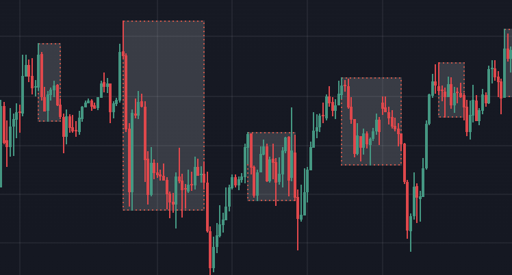
The Darvas Box Breakout Strategy defines a box using a series of rejection candles after a high or low, triggering a trade when the price breaks out of this range. Either way, we need a signal to start collecting feature data and predicting future outcomes. So, we’ll set the trigger as the moment the price breaks out of the lower or upper range. This function detects whether there is a Darvas box for a given look back period and confirmation candle amount, assigns the high/low range value to variables, and plots the box on the chart.
double high;
double low;
bool boxFormed = false;

bool DetectDarvasBox(int n = 100, int M = 3)
{
   // Clear previous Darvas box objects
   for (int k = ObjectsTotal(0, 0, -1) - 1; k >= 0; k--)
   {
      string name = ObjectName(0, k);
      if (StringFind(name, "DarvasBox_") == 0)
         ObjectDelete(0, name);
   }
   bool current_box_active = false;
   // Start checking from the oldest bar within the lookback period
   for (int i = M+1; i <= n; i++)
   {
      // Get high of current bar and previous bar
      double high_current = iHigh(_Symbol, PERIOD_CURRENT, i);
      double high_prev = iHigh(_Symbol, PERIOD_CURRENT, i + 1);
      // Check for a new high
      if (high_current > high_prev)
      {
         // Check if the next M bars do not exceed the high
         bool pullback = true;
         for (int k = 1; k <= M; k++)
         {
            if (i - k < 0) // Ensure we don't go beyond available bars
            {
               pullback = false;
               break;
            }
            double high_next = iHigh(_Symbol, PERIOD_CURRENT, i - k);
            if (high_next > high_current)
            {
               pullback = false;
               break;
            }
         }

         // If pullback condition is met, define the box
         if (pullback)
         {
            double top = high_current;
            double bottom = iLow(_Symbol, PERIOD_CURRENT, i);

            // Find the lowest low over the bar and the next M bars
            for (int k = 1; k <= M; k++)
            {
               double low_next = iLow(_Symbol, PERIOD_CURRENT, i - k);
               if (low_next < bottom)
                  bottom = low_next;
            }

            // Check for breakout from i - M - 1 to the current bar (index 0)
            int j = i - M - 1;
            while (j >= 0)
            {
               double close_j = iClose(_Symbol, PERIOD_CURRENT, j);
               if (close_j > top || close_j < bottom)
                  break; // Breakout found
               j--;
            }
            j++; // Adjust to the bar after breakout (or 0 if no breakout)

            // Create a unique object name
            string obj_name = "DarvasBox_" + IntegerToString(i);

            // Plot the box
            datetime time_start = iTime(_Symbol, PERIOD_CURRENT, i);
            datetime time_end;
            if (j > 0)
            {
               // Historical box: ends at breakout
               time_end = iTime(_Symbol, PERIOD_CURRENT, j);
            }
            else
            {
               // Current box: extends to the current bar
               time_end = iTime(_Symbol, PERIOD_CURRENT, 0);
               current_box_active = true;
            }
            high = top;
            low = bottom;
            ObjectCreate(0, obj_name, OBJ_RECTANGLE, 0, time_start, top, time_end, bottom);
            ObjectSetInteger(0, obj_name, OBJPROP_COLOR, clrBlue);
            ObjectSetInteger(0, obj_name, OBJPROP_STYLE, STYLE_SOLID);
            ObjectSetInteger(0, obj_name, OBJPROP_WIDTH, 1);
            boxFormed = true;

            // Since we're only plotting the most recent box, break after finding it
            break;
         }
      }
   }

   return current_box_active;
}
Here are some examples of the Darvas box on a chart:
Compared to using it as a filter, this method has downsides. We’d need to predict balanced outcomes with equal probabilities, like whether the next 10 bars will be higher or lower, or if the price will hit 10 pips up or down first. Another drawback is that we lose the built-in edge of a backbone strategy—the advantage depends entirely on the model’s predictive power. On the plus side, you’re not limited by the samples a backbone strategy provides only when it triggers, giving you a larger initial sample size and greater potential upside. We implement the trading logic in the onTick() function like this:
input int checkBar = 30;
input int lookBack = 100;
input int countMax = 10;

void OnTick()
  {
  int bars = iBars(_Symbol,PERIOD_CURRENT);

  if (barsTotal!= bars){
     barsTotal = bars;
     boxFormed = false;
     bool NotInPosition = true;

     lastClose = iClose(_Symbol, PERIOD_CURRENT, 1);
     lastlastClose = iClose(_Symbol,PERIOD_CURRENT,2);

     for(int i = 0; i<PositionsTotal(); i++){
         ulong pos = PositionGetTicket(i);
         string symboll = PositionGetSymbol(i);
         if(PositionGetInteger(POSITION_MAGIC) == Magic&&symboll== _Symbol)NotInPosition = false;}
            /*count++;
            if(count >=countMax ){
              trade.PositionClose(pos);
              count = 0;}
            }}*/
     DetectDarvasBox(lookBack,checkBar);
     if (NotInPosition&&boxFormed&&((lastlastClose<high&&lastClose>high)||(lastClose<low&&lastlastClose>low)))executeBuy();
    }
 }
For this strategy, using the same take profit and stop loss size is more consistent than tracking the next 10 bars’ results. The former ties our prediction directly to the final profit, while the latter adds uncertainty with varying returns over each 10-bar period. It’s worth noting that we use take profit and stop loss as a percentage of price, making it more adaptable across different assets and better suited for trending assets like gold or indices. Readers can test the alternative by uncommenting the commented code and removing take profit and stop loss from the buy function.
For the features data used to predict outcomes, I selected the past three normalized returns, the normalized distance from the range high and range low, and some common stationary indicators. We store this data in a multi-array, which is then saved to a CSV file using the CFileCSV class from an included file. Ensure all timeframes and symbols are set as listed below to easily switch between timeframes and assets.string data[50000][12]; int indexx = 0; void getData(){ double close = iClose(_Symbol,PERIOD_CURRENT,1); double close2 = iClose(_Symbol,PERIOD_CURRENT,2); double close3 = iClose(_Symbol,PERIOD_CURRENT,3); double stationary = 1000*(close-iOpen(_Symbol,PERIOD_CURRENT,1))/close; double stationary2 = 1000*(close2-iOpen(_Symbol,PERIOD_CURRENT,2))/close2; double stationary3 = 1000*(close3-iOpen(_Symbol,PERIOD_CURRENT,3))/close3; double highDistance = 1000*(close-high)/close; double lowDistance = 1000*(close-low)/close; double boxSize = 1000*(high-low)/close; double adx[]; // Average Directional Movement Index double wilder[]; // Average Directional Movement Index by Welles Wilder double dm[]; // DeMarker double rsi[]; // Relative Strength Index double rvi[]; // Relative Vigor Index double sto[]; // Stochastic Oscillator CopyBuffer(handleAdx, 0, 1, 1, adx); // Average Directional Movement Index CopyBuffer(handleWilder, 0, 1, 1, wilder); // Average Directional Movement Index by Welles Wilder CopyBuffer(handleDm, 0, 1, 1, dm); // DeMarker CopyBuffer(handleRsi, 0, 1, 1, rsi); // Relative Strength Index CopyBuffer(handleRvi, 0, 1, 1, rvi); // Relative Vigor Index CopyBuffer(handleSto, 0, 1, 1, sto); // Stochastic Oscillator //2 means 2 decimal places data[indexx][0] = DoubleToString(adx[0], 2); // Average Directional Movement Index data[indexx][1] = DoubleToString(wilder[0], 2); // Average Directional Movement Index by Welles Wilder data[indexx][2] = DoubleToString(dm[0], 2); // DeMarker data[indexx][3] = DoubleToString(rsi[0], 2); // Relative Strength Index data[indexx][4] = DoubleToString(rvi[0], 2); // Relative Vigor Index data[indexx][5] = DoubleToString(sto[0], 2); // Stochastic Oscillator data[indexx][6] = DoubleToString(stationary,2); data[indexx][7] = DoubleToString(boxSize,2); data[indexx][8] = DoubleToString(stationary2,2); data[indexx][9] = DoubleToString(stationary3,2); data[indexx][10] = DoubleToString(highDistance,2); data[indexx][11] = DoubleToString(lowDistance,2); indexx++; }
The final code for the data fetching expert advisor will look like this:
#include <Trade/Trade.mqh>
CTrade trade;
#include <FileCSV.mqh>
CFileCSV csvFile;
string fileName = "box.csv";
string headers[] = {
    "Average Directional Movement Index",
    "Average Directional Movement Index by Welles Wilder",
    "DeMarker",
    "Relative Strength Index",
    "Relative Vigor Index",
    "Stochastic Oscillator",
    "Stationary",
    "Box Size",
    "Stationary2",
    "Stationary3",
    "Distance High",
    "Distance Low"
};

input double lott = 0.01;
input int Magic = 0;
input int checkBar = 30;
input int lookBack = 100;
input int countMax = 10;
input double slp = 0.003;
input double tpp = 0.003;
input bool saveData = true;

string data[50000][12];
int indexx = 0;
int barsTotal = 0;
int count = 0;
double high;
double low;
bool boxFormed = false;
double lastClose;
double lastlastClose;

int handleAdx;     // Average Directional Movement Index - 3
int handleWilder;  // Average Directional Movement Index by Welles Wilder - 3
int handleDm;      // DeMarker - 1
int handleRsi;     // Relative Strength Index - 1
int handleRvi;     // Relative Vigor Index - 2
int handleSto;     // Stochastic Oscillator - 2

int OnInit()
  {
   trade.SetExpertMagicNumber(Magic);
handleAdx=iADX(_Symbol,PERIOD_CURRENT,14);//Average Directional Movement Index - 3
handleWilder=iADXWilder(_Symbol,PERIOD_CURRENT,14);//Average Directional Movement Index by Welles Wilder - 3
handleDm=iDeMarker(_Symbol,PERIOD_CURRENT,14);//DeMarker - 1
handleRsi=iRSI(_Symbol,PERIOD_CURRENT,14,PRICE_CLOSE);//Relative Strength Index - 1
handleRvi=iRVI(_Symbol,PERIOD_CURRENT,10);//Relative Vigor Index - 2
handleSto=iStochastic(_Symbol,PERIOD_CURRENT,5,3,3,MODE_SMA,STO_LOWHIGH);//Stochastic Oscillator - 2
   return(INIT_SUCCEEDED);
  }

void OnDeinit(const int reason)
  {
   if (!saveData) return;
   if(csvFile.Open(fileName, FILE_WRITE|FILE_ANSI))
     {
      //Write the header
      csvFile.WriteHeader(headers);
      //Write data rows
      csvFile.WriteLine(data);
      //Close the file
      csvFile.Close();
     }
   else
     {
      Print("File opening error!");
     }
  }

void OnTick()
  {
  int bars = iBars(_Symbol,PERIOD_CURRENT);

  if (barsTotal!= bars){
     barsTotal = bars;
     boxFormed = false;
     bool NotInPosition = true;

     lastClose = iClose(_Symbol, PERIOD_CURRENT, 1);
     lastlastClose = iClose(_Symbol,PERIOD_CURRENT,2);

     for(int i = 0; i<PositionsTotal(); i++){
         ulong pos = PositionGetTicket(i);
         string symboll = PositionGetSymbol(i);
         if(PositionGetInteger(POSITION_MAGIC) == Magic&&symboll== _Symbol)NotInPosition = false;}
            /*count++;
            if(count >=countMax ){
              trade.PositionClose(pos);
              count = 0;}
            }}*/
     DetectDarvasBox(lookBack,checkBar);
     if (NotInPosition&&boxFormed&&((lastlastClose<high&&lastClose>high)||(lastClose<low&&lastlastClose>low)))executeBuy();
    }
 }

void executeBuy() {
       double ask = SymbolInfoDouble(_Symbol, SYMBOL_ASK);
       ask = NormalizeDouble(ask,_Digits);
       double sl = lastClose*(1-slp);
       double tp = lastClose*(1+tpp);
       trade.Buy(lott,_Symbol,ask,sl,tp);
       if(PositionsTotal()>0)getData();
}

bool DetectDarvasBox(int n = 100, int M = 3)
{
   // Clear previous Darvas box objects
   for (int k = ObjectsTotal(0, 0, -1) - 1; k >= 0; k--)
   {
      string name = ObjectName(0, k);
      if (StringFind(name, "DarvasBox_") == 0)
         ObjectDelete(0, name);
   }
   bool current_box_active = false;
   // Start checking from the oldest bar within the lookback period
   for (int i = M+1; i <= n; i++)
   {
      // Get high of current bar and previous bar
      double high_current = iHigh(_Symbol, PERIOD_CURRENT, i);
      double high_prev = iHigh(_Symbol, PERIOD_CURRENT, i + 1);
      // Check for a new high
      if (high_current > high_prev)
      {
         // Check if the next M bars do not exceed the high
         bool pullback = true;
         for (int k = 1; k <= M; k++)
         {
            if (i - k < 0) // Ensure we don't go beyond available bars
            {
               pullback = false;
               break;
            }
            double high_next = iHigh(_Symbol, PERIOD_CURRENT, i - k);
            if (high_next > high_current)
            {
               pullback = false;
               break;
            }
         }

         // If pullback condition is met, define the box
         if (pullback)
         {
            double top = high_current;
            double bottom = iLow(_Symbol, PERIOD_CURRENT, i);

            // Find the lowest low over the bar and the next M bars
            for (int k = 1; k <= M; k++)
            {
               double low_next = iLow(_Symbol, PERIOD_CURRENT, i - k);
               if (low_next < bottom)
                  bottom = low_next;
            }

            // Check for breakout from i - M - 1 to the current bar (index 0)
            int j = i - M - 1;
            while (j >= 0)
            {
               double close_j = iClose(_Symbol, PERIOD_CURRENT, j);
               if (close_j > top || close_j < bottom)
                  break; // Breakout found
               j--;
            }
            j++; // Adjust to the bar after breakout (or 0 if no breakout)

            // Create a unique object name
            string obj_name = "DarvasBox_" + IntegerToString(i);

            // Plot the box
            datetime time_start = iTime(_Symbol, PERIOD_CURRENT, i);
            datetime time_end;
            if (j > 0)
            {
               // Historical box: ends at breakout
               time_end = iTime(_Symbol, PERIOD_CURRENT, j);
            }
            else
            {
               // Current box: extends to the current bar
               time_end = iTime(_Symbol, PERIOD_CURRENT, 0);
               current_box_active = true;
            }
            high = top;
            low = bottom;
            ObjectCreate(0, obj_name, OBJ_RECTANGLE, 0, time_start, top, time_end, bottom);
            ObjectSetInteger(0, obj_name, OBJPROP_COLOR, clrBlue);
            ObjectSetInteger(0, obj_name, OBJPROP_STYLE, STYLE_SOLID);
            ObjectSetInteger(0, obj_name, OBJPROP_WIDTH, 1);
            boxFormed = true;

            // Since we're only plotting the most recent box, break after finding it
            break;
         }
      }
   }

   return current_box_active;
}

void getData(){
double close = iClose(_Symbol,PERIOD_CURRENT,1);
double close2 = iClose(_Symbol,PERIOD_CURRENT,2);
double close3 = iClose(_Symbol,PERIOD_CURRENT,3);
double stationary = 1000*(close-iOpen(_Symbol,PERIOD_CURRENT,1))/close;
double stationary2 = 1000*(close2-iOpen(_Symbol,PERIOD_CURRENT,2))/close2;
double stationary3 = 1000*(close3-iOpen(_Symbol,PERIOD_CURRENT,3))/close3;
double highDistance = 1000*(close-high)/close;
double lowDistance = 1000*(close-low)/close;
double boxSize = 1000*(high-low)/close;
double adx[];       // Average Directional Movement Index
double wilder[];    // Average Directional Movement Index by Welles Wilder
double dm[];        // DeMarker
double rsi[];       // Relative Strength Index
double rvi[];       // Relative Vigor Index
double sto[];       // Stochastic Oscillator

CopyBuffer(handleAdx, 0, 1, 1, adx);         // Average Directional Movement Index
CopyBuffer(handleWilder, 0, 1, 1, wilder);   // Average Directional Movement Index by Welles Wilder
CopyBuffer(handleDm, 0, 1, 1, dm);           // DeMarker
CopyBuffer(handleRsi, 0, 1, 1, rsi);         // Relative Strength Index
CopyBuffer(handleRvi, 0, 1, 1, rvi);         // Relative Vigor Index
CopyBuffer(handleSto, 0, 1, 1, sto);         // Stochastic Oscillator

//2 means 2 decimal places
data[indexx][0] = DoubleToString(adx[0], 2);      // Average Directional Movement Index
data[indexx][1] = DoubleToString(wilder[0], 2);   // Average Directional Movement Index by Welles Wilder
data[indexx][2] = DoubleToString(dm[0], 2);       // DeMarker
data[indexx][3] = DoubleToString(rsi[0], 2);     // Relative Strength Index
data[indexx][4] = DoubleToString(rvi[0], 2);     // Relative Vigor Index
data[indexx][5] = DoubleToString(sto[0], 2);     // Stochastic Oscillator
data[indexx][6] = DoubleToString(stationary,2);
data[indexx][7] = DoubleToString(boxSize,2);
data[indexx][8] = DoubleToString(stationary2,2);
data[indexx][9] = DoubleToString(stationary3,2);
data[indexx][10] = DoubleToString(highDistance,2);
data[indexx][11] = DoubleToString(lowDistance,2);
indexx++;
}
We intend to trade this strategy on the XAUUSD 15-minute timeframe due to the asset’s solid volatility, and because 15 minutes strikes a balance between reduced noise and generating a higher number of samples. A typical trade would look like this:
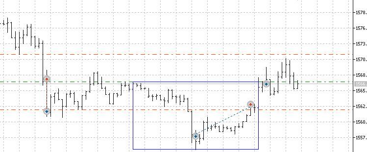
We use the data from 2020-2024 as training data and validation data, and we will test the result on 2024-2025 in MetaTrader 5 terminal later. After running this EA in the strategy tester, the CSV file will be saved in the /Tester/Agent-sth000 directory upon EA deinitialization.
Also, right click to get the backtest excel report like this:
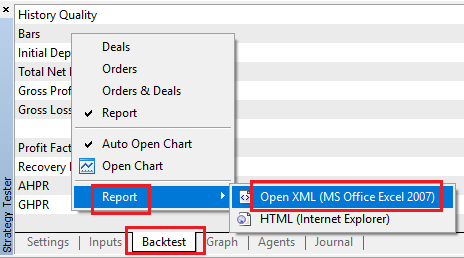
Please note the row number of the "Deals" row, which we will use as input later.

After that, we train our model in python.
The model we selected for this article is a decision tree-based model, ideal for classification problems, just like the one we used in this article.
import pandas as pd

# Replace 'your_file.xlsx' with the path to your file
input_file = 'box.xlsx'

# Load the Excel file and skip the first {skiprows} rows
data1 = pd.read_excel(input_file, skiprows=4417)

# Select the 'profit' column (assumed to be 'Unnamed: 10') and filter rows as per your instructions
profit_data = data1["Profit"][1:-1]
profit_data = profit_data[profit_data.index % 2 == 0]  # Filter for rows with odd indices
profit_data = profit_data.reset_index(drop=True)  # Reset index
# Convert to float, then apply the condition to set values to 1 if > 0, otherwise to 0
profit_data = pd.to_numeric(profit_data, errors='coerce').fillna(0)  # Convert to float, replacing NaN with 0
profit_data = profit_data.apply(lambda x: 1 if x > 0 else 0)  # Apply condition

# Load the CSV file with semicolon separator
file_path = 'box.csv'
data2 = pd.read_csv(file_path, sep=';')

# Drop rows with any missing or incomplete values
data2.dropna(inplace=True)

# Drop any duplicate rows if present
data2.drop_duplicates(inplace=True)

# Convert non-numeric columns to numerical format
for col in data2.columns:
    if data2[col].dtype == 'object':
        # Convert categorical to numerical using label encoding
        data2[col] = data2[col].astype('category').cat.codes

# Ensure all remaining columns are numeric and cleanly formatted for CatBoost
data2 = data2.apply(pd.to_numeric, errors='coerce')
data2.dropna(inplace=True)  # Drop any rows that might still contain NaNs after conversion

# Merge the two DataFrames on the index
merged_data = pd.merge(profit_data, data2, left_index=True, right_index=True, how='inner')

# Save the merged data to a new CSV file
output_csv_path = 'merged_data.csv'
merged_data.to_csv(output_csv_path)

print(f"Merged data saved to {output_csv_path}")
We use this code to label the Excel report, assigning a 1 to trades with positive profit and a 0 to those without. Then, we combine it with the feature data collected from the data-fetching EA’s CSV file. Keep in mind that the skiprow value matches the row number of "Deals."
import numpy as np
import pandas as pd
import warnings
warnings.filterwarnings("ignore")
data = pd.read_csv("merged_data.csv",index_col=0)

XX = data.drop(columns=['Profit'])
yy = data['Profit']
y = yy.values
X = XX.values
pd.DataFrame(X,y)
Next, we assign the label array to the y variable and the feature data frame to the X variable.
import numpy as np
import pandas as pd
import warnings
import seaborn as sns
warnings.filterwarnings("ignore")
from sklearn.model_selection import train_test_split
import catboost as cb
from sklearn.metrics import roc_curve, roc_auc_score
import matplotlib.pyplot as plt

# Split data
X_train, X_test, y_train, y_test = train_test_split(X, y, test_size=0.1, shuffle=False)

# Identify categorical features
cat_feature_indices = [i for i, col in enumerate(XX.columns) if XX[col].dtype == 'object']

# Train CatBoost classifier
model = cb.CatBoostClassifier(
    iterations=5000,             # Number of trees (similar to n_estimators)
    learning_rate=0.02,          # Learning rate
    depth=5,                    # Depth of each tree
    l2_leaf_reg=5,
    bagging_temperature=1,
    early_stopping_rounds=50,
    loss_function='Logloss',    # Use 'MultiClass' if it's a multi-class problem
    verbose=1000)
model.fit(X_train, y_train, cat_features=cat_feature_indices)
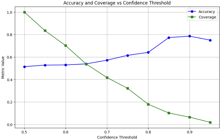
Then, we split the data 9:1 into training and validation sets and start training the model. The default setting for the train-test split function in sklearn includes shuffling, which isn’t ideal for time series data, so be sure to set shuffle=False in the parameters. It’s a good idea to tweak the hyperparameters to avoid overfitting or underfitting, depending on your sample size. Personally, I’ve found that stopping the iteration around 0.1 log loss works well.
import numpy as np
from sklearn.metrics import roc_curve, roc_auc_score
import matplotlib.pyplot as plt

# Assuming you already have y_test, X_test, and model defined
# Predict probabilities
y_prob = model.predict_proba(X_test)[:, 1]  # Probability for positive class

# Compute ROC curve and AUC (for reference)
fpr, tpr, thresholds = roc_curve(y_test, y_prob)
auc_score = roc_auc_score(y_test, y_prob)
print(f"AUC Score: {auc_score:.2f}")

# Define confidence thresholds to test (e.g., 50%, 60%, 70%, etc.)
confidence_thresholds = np.arange(0.5, 1.0, 0.05)  # From 50% to 95% in steps of 5%
accuracies = []
coverage = []  # Fraction of samples classified at each threshold

for thresh in confidence_thresholds:
    # Classify only when probability is >= thresh (positive) or <= (1 - thresh) (negative)
    y_pred_confident = np.where(y_prob >= thresh, 1, np.where(y_prob <= (1 - thresh), 0, -1))

    # Filter out unclassified samples (where y_pred_confident == -1)
    mask = y_pred_confident != -1
    y_test_confident = y_test[mask]
    y_pred_confident = y_pred_confident[mask]

    # Calculate accuracy and coverage
    if len(y_test_confident) > 0:  # Avoid division by zero
        acc = np.mean(y_pred_confident == y_test_confident)
        cov = len(y_test_confident) / len(y_test)
    else:
        acc = 0
        cov = 0

    accuracies.append(acc)
    coverage.append(cov)

# Plot Accuracy vs Confidence Threshold
plt.figure(figsize=(10, 6))
plt.plot(confidence_thresholds, accuracies, marker='o', label='Accuracy', color='blue')
plt.plot(confidence_thresholds, coverage, marker='s', label='Coverage', color='green')
plt.xlabel('Confidence Threshold')
plt.ylabel('Metric Value')
plt.title('Accuracy and Coverage vs Confidence Threshold')
plt.legend(loc='best')
plt.grid(True)
plt.show()

# Also show the original ROC curve for reference
plt.figure(figsize=(8, 6))
plt.plot(fpr, tpr, label=f'ROC Curve (AUC = {auc_score:.2f})', color='blue')
plt.plot([0, 1], [0, 1], 'k--', label='Random Guess')
plt.xlabel('False Positive Rate')
plt.ylabel('True Positive Rate')
plt.title('Receiver Operating Characteristic (ROC) Curve')
plt.legend(loc='lower right')
plt.grid(True)
plt.show()
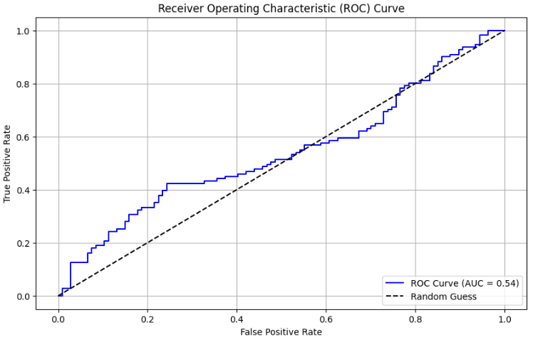
We then plot the result visualizations to check the validation test. In the typical train-validate-test approach, the validation step helps pick the best hyperparameters and initially assesses if the trained model has predictive power. It acts as a buffer before moving to the final test.
# Feature importance
feature_importance = model.get_feature_importance()
importance_df = pd.DataFrame({
    'feature': XX.columns,
    'importance': feature_importance
}).sort_values('importance', ascending=False)
print("Feature Importances:")
print(importance_df)
plt.figure(figsize=(10, 6))
sns.barplot(x='importance', y='feature', data=importance_df)
plt.title(' Feature Importance')
plt.xlabel('Importance')
plt.ylabel('Feature')
x = 100/len(XX.columns)
plt.axvline(x,color = 'red', linestyle = '--')
plt.show()
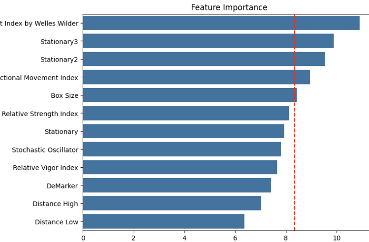
This block of code will plot out the feature importance as well as the median line. There are many ways to define feature importance in the field of machine learning, such as:
- Tree-Based Importance: Measures impurity reduction (e.g., Gini) in decision trees or ensembles like Random Forest and XGBoost.
- Permutation Importance: Assesses performance drop when a feature’s values are shuffled.
- SHAP Values: Calculates a feature’s contribution to predictions based on Shapley values.
- Coefficient Magnitude: Uses the absolute value of coefficients in linear models.
In our example, we’re using CatBoost, a decision tree-based model. Feature importance shows how much disorder (impurity) each feature reduces when used to split the decision tree in the in-sample data. It’s key to realize that while picking the most important features as your final set can often boost your model’s efficiency, it doesn’t always improve predictability for these reasons:
- The importance of features is calculated from the in-sample data, unaware of the out-of-sample data.
- Feature importance depends on the other features being considered. If most of your chosen features lack predictive power, cutting the weakest ones won’t help.
- The importance reflects how effectively a feature splits the tree, not necessarily how critical it is to the final decision outcome.
These insights hit me when I unexpectedly discovered that picking the least important features actually boosted the out-of-sample accuracy. But generally, choosing the most important features and cutting the less important ones helps lighten the model and likely improves the accuracy overall.
from onnx.helper import get_attribute_value
import onnxruntime as rt
from skl2onnx import convert_sklearn, update_registered_converter
from skl2onnx.common.shape_calculator import (
    calculate_linear_classifier_output_shapes,
)  # noqa
from skl2onnx.common.data_types import (
    FloatTensorType,
    Int64TensorType,
    guess_tensor_type,
)
from skl2onnx._parse import _apply_zipmap, _get_sklearn_operator_name
from catboost import CatBoostClassifier
from catboost.utils import convert_to_onnx_object

def skl2onnx_parser_castboost_classifier(scope, model, inputs, custom_parsers=None):

    options = scope.get_options(model, dict(zipmap=True))
    no_zipmap = isinstance(options["zipmap"], bool) and not options["zipmap"]

    alias = _get_sklearn_operator_name(type(model))
    this_operator = scope.declare_local_operator(alias, model)
    this_operator.inputs = inputs

    label_variable = scope.declare_local_variable("label", Int64TensorType())
    prob_dtype = guess_tensor_type(inputs[0].type)
    probability_tensor_variable = scope.declare_local_variable(
        "probabilities", prob_dtype
    )
    this_operator.outputs.append(label_variable)
    this_operator.outputs.append(probability_tensor_variable)
    probability_tensor = this_operator.outputs

    if no_zipmap:
        return probability_tensor

    return _apply_zipmap(
        options["zipmap"], scope, model, inputs[0].type, probability_tensor
    )

def skl2onnx_convert_catboost(scope, operator, container):
    """
    CatBoost returns an ONNX graph with a single node.
    This function adds it to the main graph.
    """
    onx = convert_to_onnx_object(operator.raw_operator)
    opsets = {d.domain: d.version for d in onx.opset_import}
    if "" in opsets and opsets[""] >= container.target_opset:
        raise RuntimeError("CatBoost uses an opset more recent than the target one.")
    if len(onx.graph.initializer) > 0 or len(onx.graph.sparse_initializer) > 0:
        raise NotImplementedError(
            "CatBoost returns a model initializers. This option is not implemented yet."
        )
    if (
        len(onx.graph.node) not in (1, 2)
        or not onx.graph.node[0].op_type.startswith("TreeEnsemble")
        or (len(onx.graph.node) == 2 and onx.graph.node[1].op_type != "ZipMap")
    ):
        types = ", ".join(map(lambda n: n.op_type, onx.graph.node))
        raise NotImplementedError(
            f"CatBoost returns {len(onx.graph.node)} != 1 (types={types}). "
            f"This option is not implemented yet."
        )
    node = onx.graph.node[0]
    atts = {}
    for att in node.attribute:
        atts[att.name] = get_attribute_value(att)
    container.add_node(
        node.op_type,
        [operator.inputs[0].full_name],
        [operator.outputs[0].full_name, operator.outputs[1].full_name],
        op_domain=node.domain,
        op_version=opsets.get(node.domain, None),
        **atts,
    )

update_registered_converter(
    CatBoostClassifier,
    "CatBoostCatBoostClassifier",
    calculate_linear_classifier_output_shapes,
    skl2onnx_convert_catboost,
    parser=skl2onnx_parser_castboost_classifier,
    options={"nocl": [True, False], "zipmap": [True, False, "columns"]},
)
model_onnx = convert_sklearn(
    model,
    "catboost",
    [("input", FloatTensorType([None, X.shape[1]]))],
    target_opset={"": 12, "ai.onnx.ml": 2},
)

# And save.
with open("box2024.onnx", "wb") as f:
    f.write(model_onnx.SerializeToString())
Finally, we export the ONNX file and save it to the MQL5/Files directory.
Now, let's go back to the MetaTrader 5 code editor to create the trading EA.
We just need to tweak the original data-fetching EA by importing some include files to handle the CatBoost model.
#resource "\\Files\\box2024.onnx" as uchar catboost_onnx[]
#include <CatOnnx.mqh>
CCatBoost cat_boost;
string data[1][12];
vector xx;
vector prob;
Then, we’ll adjust the getData() function to return a vector.
vector getData(){
double close = iClose(_Symbol,PERIOD_CURRENT,1);
double close2 = iClose(_Symbol,PERIOD_CURRENT,2);
double close3 = iClose(_Symbol,PERIOD_CURRENT,3);
double stationary = 1000*(close-iOpen(_Symbol,PERIOD_CURRENT,1))/close;
double stationary2 = 1000*(close2-iOpen(_Symbol,PERIOD_CURRENT,2))/close2;
double stationary3 = 1000*(close3-iOpen(_Symbol,PERIOD_CURRENT,3))/close3;
double highDistance = 1000*(close-high)/close;
double lowDistance = 1000*(close-low)/close;
double boxSize = 1000*(high-low)/close;
double adx[];       // Average Directional Movement Index
double wilder[];    // Average Directional Movement Index by Welles Wilder
double dm[];        // DeMarker
double rsi[];       // Relative Strength Index
double rvi[];       // Relative Vigor Index
double sto[];       // Stochastic Oscillator

CopyBuffer(handleAdx, 0, 1, 1, adx);         // Average Directional Movement Index
CopyBuffer(handleWilder, 0, 1, 1, wilder);   // Average Directional Movement Index by Welles Wilder
CopyBuffer(handleDm, 0, 1, 1, dm);           // DeMarker
CopyBuffer(handleRsi, 0, 1, 1, rsi);         // Relative Strength Index
CopyBuffer(handleRvi, 0, 1, 1, rvi);         // Relative Vigor Index
CopyBuffer(handleSto, 0, 1, 1, sto);         // Stochastic Oscillator

data[0][0] = DoubleToString(adx[0], 2);      // Average Directional Movement Index
data[0][1] = DoubleToString(wilder[0], 2);   // Average Directional Movement Index by Welles Wilder
data[0][2] = DoubleToString(dm[0], 2);       // DeMarker
data[0][3] = DoubleToString(rsi[0], 2);     // Relative Strength Index
data[0][4] = DoubleToString(rvi[0], 2);     // Relative Vigor Index
data[0][5] = DoubleToString(sto[0], 2);     // Stochastic Oscillator
data[0][6] = DoubleToString(stationary,2);
data[0][7] = DoubleToString(boxSize,2);
data[0][8] = DoubleToString(stationary2,2);
data[0][9] = DoubleToString(stationary3,2);
data[0][10] = DoubleToString(highDistance,2);
data[0][11] = DoubleToString(lowDistance,2);

vector features(12);
   for(int i = 0; i < 12; i++)
    {
      features[i] = StringToDouble(data[0][i]);
    }
    return features;
}
The final trading logic in the OnTick() function will end up looking like this:
void OnTick()
  {
  int bars = iBars(_Symbol,PERIOD_CURRENT);

  if (barsTotal!= bars){
     barsTotal = bars;
     boxFormed = false;
     bool NotInPosition = true;

     lastClose = iClose(_Symbol, PERIOD_CURRENT, 1);
     lastlastClose = iClose(_Symbol,PERIOD_CURRENT,2);

     for(int i = 0; i<PositionsTotal(); i++){
         ulong pos = PositionGetTicket(i);
         string symboll = PositionGetSymbol(i);
         if(PositionGetInteger(POSITION_MAGIC) == Magic&&symboll== _Symbol)NotInPosition = false;}
            /*count++;
            if(count >=countMax){
              trade.PositionClose(pos);
              count = 0;}
            }}*/
     DetectDarvasBox(lookBack,checkBar);
     if (NotInPosition&&boxFormed&&((lastlastClose<high&&lastClose>high)||(lastClose<low&&lastlastClose>low))){
        xx = getData();
        prob = cat_boost.predict_proba(xx);
        if(prob[1]>threshold)executeBuy();
        if(prob[0]>threshold)executeSell();
        }
    }
 }
In the signal logic, it first checks that no position is currently open to ensure only one trade at a time. Then, it detects if there’s a breakout on either side of the range. After that, it calls the getData() function to get the features vector. This vector is passed to the CatBoost model as input, and the model outputs the prediction confidence for each outcome into the prob array. Based on the confidence levels for each outcome, we place a trade betting on the predicted outcome. Essentially, we’re using the model to generate the buy or sell signals.
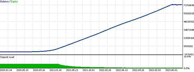
We ran a backtest on the MetaTrader 5 strategy tester using in-sample data from 2020 to 2024 to verify that our training data had no errors and that the merging of features and outcomes was correct. If everything is accurate, the equity curve should look nearly perfect, like this:
We then backtest the out-of-sample test from 2024 to 2025 to see if the strategy has profitability in the most recent period. We set the threshold to 0.7, so the model will only take a trade in a direction if the confidence level for that direction’s take-profit being hit is 70% or higher, based on the training data.
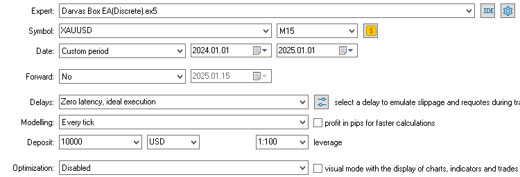

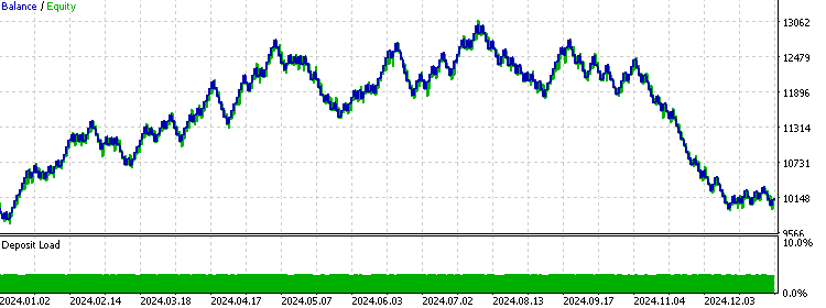
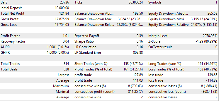
We can see that the model performed exceptionally well in the first half of the year but started to underperform as time went on. This is common with machine learning models because the edge gained from past data is often temporary, and that edge tends to erode over time. This suggests that a smaller test-train ratio might work better for future live trading implementations. Overall, the model shows some predictability, since it remained profitable even after accounting for trading costs.
Continuous Signal
In algorithmic trading, traders typically stick to a simple method of using discrete signals—either buy or sell with a fixed risk per trade. This keeps things easy to handle and better for analyzing strategy performance. Some traders have tried to refine this discrete signal method by using an additive signal, where they adjust the trade’s risk based on how strongly the strategy’s conditions are met. Continuous signals take this additive approach further, applying it to more abstract strategy conditions and producing a risk level between zero and one.
The basic idea behind this is that not all trades meeting entry criteria are equal. Some seem more likely to succeed because their signals are stronger, based on non-linear rules tied to the strategy. This can be seen as a risk management tool—bet big when confidence is high and scale back when a trade looks less promising, even if it still has a positive expected return. However, we need to remember that this adds another factor to the strategy performance, and that look-ahead bias and overfitting risks are still problematic if we are not careful during implementation.
To apply this concept in our trading EA, we first need to tweak the buy/sell functions to calculate lot size based on the risk we’re willing to lose if the stop loss is hit. The lot calculation function looks like this:
double calclots(double slpoints, string symbol, double risk)
{
   double balance = AccountInfoDouble(ACCOUNT_BALANCE);
   double riskAmount = balance* risk / 100;

   double ticksize = SymbolInfoDouble(symbol, SYMBOL_TRADE_TICK_SIZE);
   double tickvalue = SymbolInfoDouble(symbol, SYMBOL_TRADE_TICK_VALUE);
   double lotstep = SymbolInfoDouble(symbol, SYMBOL_VOLUME_STEP);

   double moneyperlotstep = slpoints / ticksize * tickvalue * lotstep;
   double lots = MathFloor(riskAmount / moneyperlotstep) * lotstep;
   lots = MathMin(lots, SymbolInfoDouble(symbol, SYMBOL_VOLUME_MAX));
   lots = MathMax(lots, SymbolInfoDouble(symbol, SYMBOL_VOLUME_MIN));
   return lots;
}
We then update the buy/sell functions so they call this calclots() function and take the risk multiplier as input:
void executeSell(double riskMultiplier) {
       double bid = SymbolInfoDouble(_Symbol, SYMBOL_BID);
       bid = NormalizeDouble(bid,_Digits);
       double sl = lastClose*(1+slp);
       double tp = lastClose*(1-tpp);
       double lots = 0.1;
       lots = calclots(slp*lastClose,_Symbol,risks*riskMultiplier);
       trade.Sell(lots,_Symbol,bid,sl,tp);
       }

void executeBuy(double riskMultiplier) {
       double ask = SymbolInfoDouble(_Symbol, SYMBOL_ASK);
       ask = NormalizeDouble(ask,_Digits);
       double sl = lastClose*(1-slp);
       double tp = lastClose*(1+tpp);
       double lots = 0.1;
       lots = calclots(slp*lastClose,_Symbol,risks*riskMultiplier);
       trade.Buy(lots,_Symbol,ask,sl,tp);
}
Since our machine learning model already outputs the confidence level, we can directly use it as the risk multiplier input. If we want to adjust how much the confidence level affects the risk for each trade, we can simply scale the confidence level up or down as needed.
if(prob[1]>threshold)executeBuy(prob[1]);
if(prob[0]>threshold)executeSell(prob[0]);
For example, if we want to amplify the significance of the confidence level differences, we could multiply the probability by itself three times. This would increase the ratio difference between probabilities, making the impact of confidence levels more pronounced.
if(prob[1]>threshold)executeBuy(prob[1]*prob[1]*prob[1]);
if(prob[0]>threshold)executeSell(prob[0]*prob[0]*prob[0]);
Now, we try to see the result in the backtest.
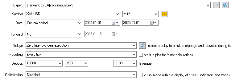
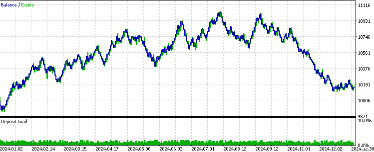
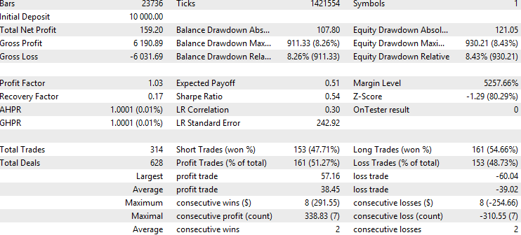
The trades taken are still the same as in the discrete signal version, but the profit factor and Sharpe ratio improved slightly. This suggests that, in this specific scenario, the continuous signal enhanced the overall performance of the out-of-sample test, which is free of look-ahead bias since we only tested once. However, it’s important to note that this approach only outperforms the fixed-risk method if the model’s prediction accuracy is higher when its confidence level is higher. Otherwise, the original fixed-risk approach might be better. Additionally, since we reduced the average lot size by applying risk multipliers between zero and one, we’d need to increase the risk variable value if we want to achieve similar total profit as before.
Multi-Timeframe Validation
Training separate machine learning models, each using a different timeframe of features to predict the same outcome, can offer a powerful way to improve trade filtering and signal generation. By having one model focus on short-term data, another on medium-term, and perhaps a third on long-term trends, you gain specialized insights that, when combined, can validate predictions more reliably than a single model. This multi-model approach can boost confidence in trade decisions by cross-checking signals, reducing the risk of acting on noise specific to one timeframe, and it supports risk management by allowing you to weigh each model’s output to adjust trade size or stops based on consensus strength.
On the flip side, this strategy can complicate the system, especially when you assign different weights to predictions from multiple models. This might introduce its own biases or errors if not carefully tuned. Each model could also overfit to its specific timeframe, missing broader market dynamics, and discrepancies between their predictions might create confusion, delaying decisions or undermining confidence.
This approach relies on two key assumptions: no look-ahead bias is introduced in the higher timeframe (we must use the last bar’s value, not the current one), and the higher timeframe model has its own predictability (it performs better than random guessing in out-of-sample tests).
To implement this, we first modify the code in the data-fetching EA by changing all the timeframes related to feature extraction to a higher timeframe, like 1-hour. This includes indicators, price calculations, and any other features used.
int OnInit()
{
   trade.SetExpertMagicNumber(Magic);
   handleAdx = iADX(_Symbol, PERIOD_H1, 14); // Average Directional Movement Index - 3
   handleWilder = iADXWilder(_Symbol, PERIOD_H1, 14); // Average Directional Movement Index by Welles Wilder - 3
   handleDm = iDeMarker(_Symbol, PERIOD_H1, 14); // DeMarker - 1
   handleRsi = iRSI(_Symbol, PERIOD_H1, 14, PRICE_CLOSE); // Relative Strength Index - 1
   handleRvi = iRVI(_Symbol, PERIOD_H1, 10); // Relative Vigor Index - 2
   handleSto = iStochastic(_Symbol, PERIOD_H1, 5, 3, 3, MODE_SMA, STO_LOWHIGH); // Stochastic Oscillator - 2
   return(INIT_SUCCEEDED);
}

void getData()
{
   double close = iClose(_Symbol, PERIOD_H1, 1);
   double close2 = iClose(_Symbol, PERIOD_H1, 2);
   double close3 = iClose(_Symbol, PERIOD_H1, 3);
   double stationary = 1000 * (close - iOpen(_Symbol, PERIOD_H1, 1)) / close;
   double stationary2 = 1000 * (close2 - iOpen(_Symbol, PERIOD_H1, 2)) / close2;
   double stationary3 = 1000 * (close3 - iOpen(_Symbol, PERIOD_H1, 3)) / close3;
}
After this, we follow the same steps as before: fetching the data, training the model, and exporting it, just like we discussed earlier.
Then, in the trading EA, we make a second function for fetching the features input, we will feed this function to the second ML model we imported to get the confidence level output.
vector getData2()
{
   double close = iClose(_Symbol, PERIOD_H1, 1);
   double close2 = iClose(_Symbol, PERIOD_H1, 2);
   double close3 = iClose(_Symbol, PERIOD_H1, 3);
   double stationary = 1000 * (close - iOpen(_Symbol, PERIOD_H1, 1)) / close;
   double stationary2 = 1000 * (close2 - iOpen(_Symbol, PERIOD_H1, 2)) / close2;
   double stationary3 = 1000 * (close3 - iOpen(_Symbol, PERIOD_H1, 3)) / close3;
   double highDistance = 1000 * (close - high) / close;
   double lowDistance = 1000 * (close - low) / close;
   double boxSize = 1000 * (high - low) / close;
   double adx[];       // Average Directional Movement Index
   double wilder[];    // Average Directional Movement Index by Welles Wilder
   double dm[];        // DeMarker
   double rsi[];       // Relative Strength Index
   double rvi[];       // Relative Vigor Index
   double sto[];       // Stochastic Oscillator

   CopyBuffer(handleAdx, 0, 1, 1, adx);         // Average Directional Movement Index
   CopyBuffer(handleWilder, 0, 1, 1, wilder);   // Average Directional Movement Index by Welles Wilder
   CopyBuffer(handleDm, 0, 1, 1, dm);           // DeMarker
   CopyBuffer(handleRsi, 0, 1, 1, rsi);         // Relative Strength Index
   CopyBuffer(handleRvi, 0, 1, 1, rvi);         // Relative Vigor Index
   CopyBuffer(handleSto, 0, 1, 1, sto);         // Stochastic Oscillator

   data[0][0] = DoubleToString(adx[0], 2);      // Average Directional Movement Index
   data[0][1] = DoubleToString(wilder[0], 2);   // Average Directional Movement Index by Welles Wilder
   data[0][2] = DoubleToString(dm[0], 2);       // DeMarker
   data[0][3] = DoubleToString(rsi[0], 2);     // Relative Strength Index
   data[0][4] = DoubleToString(rvi[0], 2);     // Relative Vigor Index
   data[0][5] = DoubleToString(sto[0], 2);     // Stochastic Oscillator
   data[0][6] = DoubleToString(stationary, 2);
   data[0][7] = DoubleToString(boxSize, 2);
   data[0][8] = DoubleToString(stationary2, 2);
   data[0][9] = DoubleToString(stationary3, 2);
   data[0][10] = DoubleToString(highDistance, 2);
   data[0][11] = DoubleToString(lowDistance, 2);

   vector features(12);
   for(int i = 0; i < 12; i++)
   {
      features[i] = StringToDouble(data[0][i]);
   }
   return features;
}
Assume we want to assign the same weight to the two model's output, we simply take the average of their output and see it as the single output we used before.
if (NotInPosition&&boxFormed&&((lastlastClose<high&&lastClose>high)||(lastClose<low&&lastlastClose>low))){
        xx = getData();
        xx2 = getData2();
        prob = cat_boost.predict_proba(xx);
        prob2 = cat_boost.predict_proba(xx2);
        double probability_buy = (prob[1]+prob2[1])/2;
        double probability_sell = (prob[0]+prob2[0])/2;

        if(probability_buy>threshold)executeBuy(probability_buy);
        if(probability_sell>threshold)executeSell(probability_sell);
        }
    }
With these two variables calculated as above, we can now combine them into a single confidence level and use it for validation, following the same approach we used earlier.
Conclusion
In this article, we first explored the idea of using a machine learning model as a signal generator instead of a filter, demonstrated through a Darvas box breakout strategy. We briefly walked through the model training process and discussed the importance of confidence level thresholds and feature significance. Next, we introduced the concept of continuous signals and compared their performance to discrete signals. We found that, in this example, continuous signals improved backtest performance because the model tended to have higher prediction accuracy as confidence levels increased. Finally, we touched on the blueprint for using multiple machine learning models trained on different timeframes to validate signals together.
Overall, this article aimed to present unconventional ideas about applying machine learning models in supervised learning for CTA trading. Its goal isn’t to definitively claim which approach works best, as everything depends on the specific scenario, but rather to inspire readers to think creatively and expand on simple initial concepts. In the end, nothing is entirely new—innovation often comes from combining existing ideas to create something fresh.
File Table
| File Name | File Usage |
|---|---|
| Darvas_Box.ipynb | The Jupyter Notebook file for training the ML model |
| Darvas Box Data.mq5 | The EA for fetching data for model training |
| Darvas Box EA.mq5 | The trading EA in the article |
| CatOnnx.mqh | An include file for processing CatBoost model |
| FileCSV.mqh | An include file for saving data into CSV |
 Price Action Analysis Toolkit Development (Part 18): Introducing Quarters Theory (III) — Quarters Board
 Resampling techniques for prediction and classification assessment in MQL5
 Developing a Replay System (Part 61): Playing the service (II)
 From Novice to Expert: Support and Resistance Strength Indicator (SRSI)
- Free trading apps
- Over 8,000 signals for copying
- Economic news for exploring financial markets
You agree to website policy and terms of use
Thank you Zhou for the interesting article and code samples . for me I had to manually install some of the Python components to make it work. which may help other users !pip install catboost !pip install onnxruntime !pip install skl2onnx. on completion I can test . but if I try and load the related EA , I have returned 'Failed to set the Output[1] shape Err=5802. I am not sure where this comes from or if it is important and I am unable to work out where this is coming from . . the documentation says ERR_ONNX_NOT_SUPPORTED
Thank you for reminding. The pip install part was ignored but users do have to install the related library if they haven't already.
Your error may be caused by the dimensions used in your model training is different than the ones used in your EA. For example if you trained a model with 5 features, you ought to also input 5 features in your EA, not 4 or 6. A more detailed walk-through is in this article link . Hope this helps. If not, please provide more context.