Trend Prediction with LSTM for Trend-Following Strategies

Introduction

Long Short-Term Memory (LSTM) is a type of recurrent neural network (RNN) designed to model sequential data by effectively capturing long-term dependencies and addressing the vanishing gradient problem. In this article, we will explore how to utilize LSTM to predict future trends, enhancing the performance of trend-following strategies. The article will cover the introduction of key concepts and the motivation behind development, fetching data from MetaTrader 5, using that data to train the model in Python, integrating the machine learning model into MQL5, and reflecting on the results and future aspirations based on statistical backtesting.

Motivation

Intuitively, trend-following strategies capitalize on gains in trending markets but perform poorly in choppy markets, where the strategy ends up buying at a premium and selling at a discount. Academic research has shown that classic trend-following strategies, such as the golden cross, work across multiple markets and timeframes over long periods of history. While these strategies may not be highly profitable, they have demonstrated consistent gains. Trend-following strategies typically profit from extreme outliers, which generate significantly higher profits than the average loss. The strategy’s tight stop-loss and "let profits run" approach result in a low win rate but a high reward-to-risk ratio per trade.

LSTM (Long Short-Term Memory) is a specialized type of recurrent neural network (RNN) designed to capture long-range dependencies in sequential data. It utilizes memory cells that can maintain information over long periods, overcoming the vanishing gradient problem that typically affects traditional RNNs. This ability to store and access information from earlier in the sequence makes LSTM particularly effective for tasks like time series forecasting and trend prediction. For regression problems, LSTM can model the temporal relationships between input features and predict continuous outputs with high accuracy, making it ideal for forecasting applications.

The motivation for this article is to leverage the power of LSTM for trend regression, predicting future trends and potentially filtering out bad trades that result from low trendiness. This motivation is based on the hypothesis that trend-following strategies perform better in trendy markets compared to detrended markets.

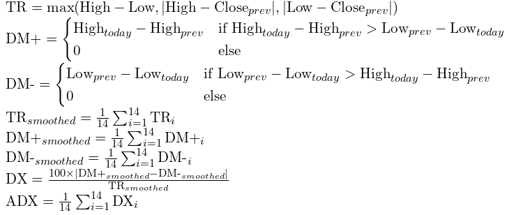
We will use the ADX (Average Directional Index) to indicate trend strength, as it is one of the most popular indicators for assessing current trendiness. We aim to predict its future value instead of using its current value, as a high ADX typically indicates that a trend has already occurred or is ending, making our entry point too late to benefit.

ADX is calculated by:

Data Preparation and Preprocessing

Before fetching data, we first need to clarify what data is required. We plan to use several features to train a regression model that predicts future ADX values. These features include the RSI, which indicates the current relative strength of the market, the return percentage of the last candle to serve as the stationary value of the close price, and ADX itself, which is directly relevant to the value we aim to predict. Note that we’ve just explained the intuition behind choosing these features. You can decide on the features yourself, but ensure they are reasonable and stationary. We plan to train the model using hourly data from 2020.1.1 to 2024.1.1 and test the model's performance from 2024.1.1-2025.1.1 as an out-of-sample test.

Now that we’ve clarified the data we want to fetch, let’s construct an expert advisor to retrieve this data.

We will use the CFileCSV class, introduced in this article, to save the array as a string in a CSV file. The code for this process is quite simple, as shown below.

#include <FileCSV.mqh>
CFileCSV csvFile;

int barsTotal = 0;
int handleRsi;
int handleAdx;
string headers[] = {
    "time",
    "ADX",
    "RSI",
    "Stationary"
};
string data[1000000][4];
int indexx = 0;
vector xx;

input string fileName = "XAU-1h-2020-2024.csv";
input bool SaveData = true;

//+------------------------------------------------------------------+
//| Expert initialization function                                   |
//+------------------------------------------------------------------+
int OnInit()
  {//Initialize model
   handleRsi = iRSI(_Symbol,PERIOD_CURRENT,14,PRICE_CLOSE);
   handleAdx = iADX(_Symbol,PERIOD_CURRENT,14);
   return(INIT_SUCCEEDED);
  }

//+------------------------------------------------------------------+
//| Expert deinitialization function                                 |
//+------------------------------------------------------------------+
void OnDeinit(const int reason)
  {
   if (!SaveData) return;
   if(csvFile.Open(fileName, FILE_WRITE|FILE_ANSI))
     {
      //Write the header
      csvFile.WriteHeader(headers);
      //Write data rows
      csvFile.WriteLine(data);
      //Close the file
      csvFile.Close();
     }
   else
     {
      Print("File opening error!");
     }

  }
  
//+------------------------------------------------------------------+
//| Expert tick function                                             |
//+------------------------------------------------------------------+
void OnTick()
  {
  int bars = iBars(_Symbol,PERIOD_CURRENT);
  
  if (barsTotal!= bars){
     barsTotal = bars;
     double rsi[];
     double adx[];
     CopyBuffer(handleAdx,0,1,1,adx);
     CopyBuffer(handleRsi,0,1,1,rsi);
     data[indexx][0] =(string)TimeTradeServer();
   data[indexx][1] = DoubleToString(adx[0], 2); 
   data[indexx][2] = DoubleToString(rsi[0], 2); 
   data[indexx][3] = DoubleToString((iClose(_Symbol,PERIOD_CURRENT,1)-iOpen(_Symbol,PERIOD_CURRENT,1))/iClose(_Symbol,PERIOD_CURRENT,1),3);
   indexx++;
   }
 }

This expert advisor (EA) is designed to track and record the values of the Relative Strength Index (RSI) and Average Directional Index (ADX) for a given symbol. The EA uses the iRSI and iADX functions to obtain the current values of RSI and ADX, and stores them along with a timestamp in a CSV file. The CSV file is created with headers for "time", "ADX", "RSI", and "Stationary". If the SaveData option is enabled, it writes the data to a file (specified by fileName) upon deinitialization. It tracks new data on each tick, and stores it when there is a change in the number of bars.

Run the Expert Advisor (EA) in the Strategy Tester with a single test. After running the test, the file should be saved in the following file path: /Tester/Agent-sth000/MQL5/Files.

Next, we move to Python for data preprocessing in preparation for training our machine learning model.

We plan to use a supervised learning approach, where the model is trained to predict a desired outcome based on labeled data. The training process involves adjusting the weights on various operations applied to the features, in order to minimize error loss and produce the final output. 

For the label, I suggest using the mean ADX value of the next 10 ADX values. This approach ensures that the trend is not already fully established by the time we enter the trade, while also preventing the trend from being too distant from the current signal. Using the mean of the next 10 ADX values is a great way to ensure that the trend remains active over the next few bars, allowing our entry to capture the profits from the upcoming directional moves.

import pandas as pd
data = pd.read_csv('XAU-1h-2020-2024.csv', sep=';')
data= data.dropna().set_index('time')
data['output'] = data['ADX'].shift(-10)
data = data[:-10]
data['output']= data['output'].rolling(window=10).mean()
data = data[9:]

This code reads the CSV file and separates the data into different columns, as the values are grouped together by a semicolon (';'). It then removes any empty rows and sets the 'time' column as the index to ensure the data is ordered chronologically for training. Next, a new column called "output" is created, which calculates the mean of the next 10 ADX values. After this, the code drops any remaining empty rows, as some rows may not have enough future ADX values to calculate the output.

Model Training

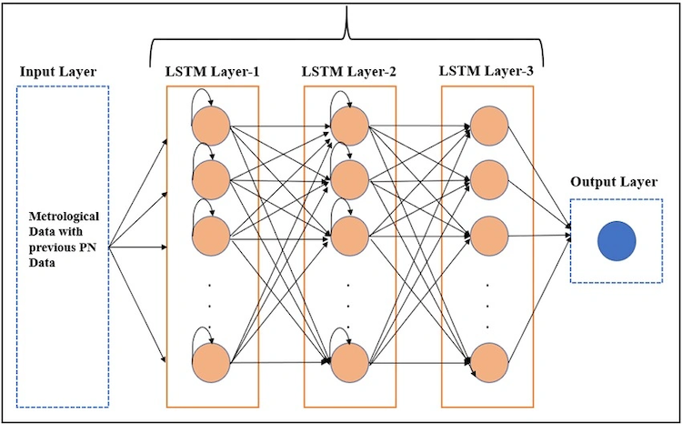
This diagram illustrates what LSTM is trying to accomplish during our training process. We want the input to have the shape (sample_amount, time_steps, feature_amount), where time_step represents how many previous time points of data we want to use to predict the next value. For example, we might use data from Monday to Thursday to predict some outcome for Friday. LSTM utilizes algorithms to identify patterns in the time series and the relationship between the features and the outcome. It creates one or more layers of neural networks, each consisting of many weight units (neurons), which apply weights to each feature and each time step to ultimately output the final prediction.

For simplicity, you could just run the following code, and it will handle the training process for you.

import numpy as np
import matplotlib.pyplot as plt
from sklearn.model_selection import train_test_split
from tensorflow.keras.models import Sequential
from tensorflow.keras.layers import LSTM, Dense

# Assume data is your DataFrame already loaded with the specified columns and a time-based index
# data.columns should include ['ADX', 'RSI', 'Stationary', 'output']

# --- Step 1: Data Preparation ---
time_step = 5

# Select features and target
features = ['ADX', 'RSI', 'Stationary']
target = 'output'

# --- Step 2: Create sequences for LSTM input ---
def create_sequences(data, target_col, time_step):
    """
    Create sequences of length time_step from the DataFrame.
    data: DataFrame of input features and target.
    target_col: Name of the target column.
    Returns: X, y arrays suitable for LSTM.
    """
    X, y = [], []
    feature_cols = data.columns.drop(target_col)
    for i in range(len(data) - time_step):
        seq_x = data.iloc[i:i+time_step][feature_cols].values
        # predict target at the next time step after the sequence
        seq_y = data.iloc[i+time_step][target_col]
        X.append(seq_x)
        y.append(seq_y)
    return np.array(X), np.array(y)

# Create sequences
X, y = create_sequences(data, target_col=target, time_step=time_step)

# --- Step 3: Split into training and evaluation sets ---
# Use a simple 80/20 split for training and evaluation
X_train, X_eval, y_train, y_eval = train_test_split(X, y, test_size=0.2, shuffle=False)

# --- Step 4: Build the LSTM model ---
n_features = len(features)  # number of features per time step

model = Sequential()
model.add(LSTM(50, input_shape=(time_step, n_features)))  # LSTM layer with 50 units
model.add(Dense(1))  # output layer for regression

model.compile(optimizer='adam', loss='mse')

model.summary()

# --- Step 5: Train the model ---
epochs = 50
batch_size = 100

history = model.fit(
    X_train, y_train,
    epochs=epochs,
    batch_size=batch_size,
    validation_data=(X_eval, y_eval)
)

Here are some important considerations when training with the above code:

1. Data Preprocessing: Ensure that your data is in time order during the preprocessing phase. Failing to do so may result in look-ahead bias when splitting the data into chunks of time_steps.

2. Train-Test Split: When splitting the data into training and test sets, do not shuffle the data. Time order must be preserved to avoid look-ahead bias.

3. Model Complexity: For time-series analysis, especially with limited data points, there's no need to construct too many layers, neurons, or epochs. Overcomplicating the model could lead to overfitting or high-bias parameters. The settings used in the example should be sufficient. 

We can then evaluate the model's accuracy using the evaluation set to assess its performance on unseen data.

# --- Step 6: Evaluate the model ---
eval_loss = model.evaluate(X_eval, y_eval)
print(f"Evaluation Loss: {eval_loss}")
# --- Step 7: Generate Predictions and Plot ---

# Generate predictions on the evaluation set
predictions = model.predict(X_eval).flatten()

# Create a plot for predictions vs actual values
plt.figure(figsize=(12, 6))
plt.plot(predictions, label='Predicted Output', color='red')
plt.plot(y_eval, label='Actual Output', color='blue')
plt.title('LSTM Predictions vs Actual Output')
plt.xlabel('Sample Index')
plt.ylabel('Output Value')
plt.legend()
plt.show()

This code should output the mean square error of the evaluation set compared with the model's prediction like this.

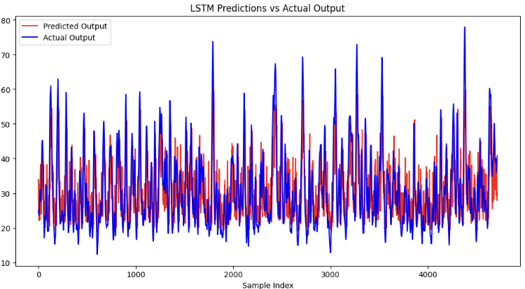
Evaluation Loss: 57.405677795410156

It is calculated by:

Where n is the sample size, yi is the predicted value for each sample, and y^i is the actual value for each evaluation outcome.

As you can see from the calculation, you can compare the model's loss to the square of the mean values of the things you're predicting to check if the relative loss is excessively high. Also, ensure that the loss is similar to that of the training sets, which indicates that the model is not overfitted to the training data.

Finally, to make the model compatible with MQL5, we want to save it in the ONNX format. Since LSTM models don't directly support ONNX transitions, we first need to save the model as a functional one, while explicitly defining the format of its input and output. After that, we can save it as an ONNX file, making it suitable for future use with MQL5.

import tensorflow as tf
import tf2onnx

# Define the input shape based on your LSTM requirements: (time_step, n_features)
time_step = 5
n_features = 3

# Create a new Keras Input layer matching the shape of your data
inputs = tf.keras.Input(shape=(time_step, n_features), name="input")

# Pass the input through your existing sequential model
outputs = model(inputs)  
functional_model = tf.keras.Model(inputs=inputs, outputs=outputs)

# Create an input signature that matches the defined input shape
input_signature = (
    tf.TensorSpec((None, time_step, n_features), dtype=tf.float32, name="input"),
)

output_path = "regression2024.onnx"

# Convert the functional model to ONNX format
onnx_model, _ = tf2onnx.convert.from_keras(
    functional_model,
    input_signature=input_signature,  # matching the input signature
    opset=15,                         
    output_path=output_path
)

print(f"Model successfully converted to ONNX at {output_path}")

Note that "None" as the input format here means the model can accept any number of samples. It will automatically output the corresponding predictions for each sample, making it flexible for varying batch sizes.

Constructing Expert Advisor

Now that we have saved the ONNX model file, we want to copy it into the /MQL5/Files directory for later use.

We go back to MetaEditor. We will build on top of a classic trend-following strategy based on the golden cross signal logic. This is the same one I implemented in my previous machine learning article. The basic logic involves two moving averages: a fast one and a slow one. A trade signal is generated when the two MAs cross, and the trade direction follows the fast moving average, hence the term "trend-following." The exit signal occurs when the price crosses the slow moving average, allowing more room for trailing stops. The complete code is as follows:

#include <Trade/Trade.mqh>
//XAU - 1h.
CTrade trade;

input int MaPeriodsFast = 15;
input int MaPeriodsSlow = 25;
input int MaPeriods = 200;
input double lott = 0.01;

ulong buypos = 0, sellpos = 0;
input int Magic = 0;
int barsTotal = 0;
int handleMaFast;
int handleMaSlow;

//+------------------------------------------------------------------+
//| Expert initialization function                                   |
//+------------------------------------------------------------------+
int OnInit()
  {
   trade.SetExpertMagicNumber(Magic);
   handleMaFast =iMA(_Symbol,PERIOD_CURRENT,MaPeriodsFast,0,MODE_SMA,PRICE_CLOSE);
   handleMaSlow =iMA(_Symbol,PERIOD_CURRENT,MaPeriodsSlow,0,MODE_SMA,PRICE_CLOSE);  
   return(INIT_SUCCEEDED);
  }

//+------------------------------------------------------------------+
//| Expert deinitialization function                                 |
//+------------------------------------------------------------------+
void OnDeinit(const int reason)
  {

  }
  
//+------------------------------------------------------------------+
//| Expert tick function                                             |
//+------------------------------------------------------------------+
void OnTick()
  {
  int bars = iBars(_Symbol,PERIOD_CURRENT);
  //Beware, the last element of the buffer list is the most recent data, not [0]
  if (barsTotal!= bars){
     barsTotal = bars;
     double maFast[];
     double maSlow[];
     CopyBuffer(handleMaFast,BASE_LINE,1,2,maFast);
     CopyBuffer(handleMaSlow,BASE_LINE,1,2,maSlow);
     double bid = SymbolInfoDouble(_Symbol, SYMBOL_BID);
     double ask = SymbolInfoDouble(_Symbol, SYMBOL_ASK);
     double lastClose = iClose(_Symbol, PERIOD_CURRENT, 1);
     //The order below matters
     if(buypos>0&& lastClose<maSlow[1]) trade.PositionClose(buypos);
     if(sellpos>0 &&lastClose>maSlow[1])trade.PositionClose(sellpos);   
     if (maFast[1]>maSlow[1]&&maFast[0]<maSlow[0]&&buypos ==sellpos)executeBuy(); 
     if(maFast[1]<maSlow[1]&&maFast[0]>maSlow[0]&&sellpos ==buypos) executeSell();
     if(buypos>0&&(!PositionSelectByTicket(buypos)|| PositionGetInteger(POSITION_MAGIC) != Magic)){
      buypos = 0;
      }
     if(sellpos>0&&(!PositionSelectByTicket(sellpos)|| PositionGetInteger(POSITION_MAGIC) != Magic)){
      sellpos = 0;
      }
    }
 }

//+------------------------------------------------------------------+
//| Expert trade transaction handling function                       |
//+------------------------------------------------------------------+
void OnTradeTransaction(const MqlTradeTransaction& trans, const MqlTradeRequest& request, const MqlTradeResult& result) {
    if (trans.type == TRADE_TRANSACTION_ORDER_ADD) {
        COrderInfo order;
        if (order.Select(trans.order)) {
            if (order.Magic() == Magic) {
                if (order.OrderType() == ORDER_TYPE_BUY) {
                    buypos = order.Ticket();
                } else if (order.OrderType() == ORDER_TYPE_SELL) {
                    sellpos = order.Ticket();
                }
            }
        }
    }
}

//+------------------------------------------------------------------+
//| Execute sell trade function                                      |
//+------------------------------------------------------------------+
void executeSell() {      
       double bid = SymbolInfoDouble(_Symbol, SYMBOL_BID);
       bid = NormalizeDouble(bid,_Digits);
       trade.Sell(lott,_Symbol,bid);  
       sellpos = trade.ResultOrder();  
       }    

//+------------------------------------------------------------------+
//| Execute buy trade function                                       |
//+------------------------------------------------------------------+
void executeBuy() {
       double ask = SymbolInfoDouble(_Symbol, SYMBOL_ASK);
       ask = NormalizeDouble(ask,_Digits);
       trade.Buy(lott,_Symbol,ask);
       buypos = trade.ResultOrder();
}

I will not elaborate further on the validation and suggestions for selecting your backbone strategy. More details can be found in my previous machine learning article, which is linked here.

Now, we will try to run our LSTM model based on this framework.

Firstly, we declare the global variables specifying the shape of our input and output, as well as two multi-arrays to store the input and output data. Additionally, we declare a model handle that will manage the process of fetching data into the model and extracting predictions from it. This setup ensures proper data flow and interaction between the model and the input/output variables.

#resource "\\Files\\regression2024.onnx" as uchar lstm_onnx[]

float data[1][5][3];
float out[1][1];
long lstmHandle = INVALID_HANDLE;
const long input_shape[] = {1,5,3};
const long output_shape[]={1,1};

Next, in the OnInit() function, we initialize the relevant indicators, such as RSI and ADX, as well as the ONNX model. During this initialization, we verify that the input shape and output shape declared in MQL5 match those specified earlier in the Python functional model. This step ensures consistency and prevents errors during model initialization, ensuring that the model can correctly process the data in the expected format.

int handleMaFast;
int handleMaSlow;
int handleAdx;     // Average Directional Movement Index - 3
int handleRsi;

//+------------------------------------------------------------------+
//| Expert initialization function                                   |
//+------------------------------------------------------------------+
int OnInit()
  {//Initialize model
   trade.SetExpertMagicNumber(Magic);
   handleMaFast =iMA(_Symbol,PERIOD_CURRENT,MaPeriodsFast,0,MODE_SMA,PRICE_CLOSE);
   handleMaSlow =iMA(_Symbol,PERIOD_CURRENT,MaPeriodsSlow,0,MODE_SMA,PRICE_CLOSE);   
   handleAdx=iADX(_Symbol,PERIOD_CURRENT,14);//Average Directional Movement Index - 3
   handleRsi = iRSI(_Symbol,PERIOD_CURRENT,14,PRICE_CLOSE);
    // Load the ONNX model
   lstmHandle = OnnxCreateFromBuffer(lstm_onnx, ONNX_DEFAULT);
   //--- specify the shape of the input data
   if(!OnnxSetInputShape(lstmHandle,0,input_shape))
     {
      Print("OnnxSetInputShape failed, error ",GetLastError());
      OnnxRelease(lstmHandle);
      return(-1);
     }
//--- specify the shape of the output data
   if(!OnnxSetOutputShape(lstmHandle,0,output_shape))
     {
      Print("OnnxSetOutputShape failed, error ",GetLastError());
      OnnxRelease(lstmHandle);
      return(-1);
     }
   if (lstmHandle == INVALID_HANDLE)
   {
      Print("Error creating model OnnxCreateFromBuffer ", GetLastError());
      return(INIT_FAILED);
   }
   return(INIT_SUCCEEDED);
  }

Next, we declare a function to update the input data with each new bar. This function loops through the time_step (in this case, 5) to store the corresponding data in the global multi-array. It converts the data to float type to ensure it meets the 32-bit requirement expected by the ONNX model. Additionally, the function ensures that the order of the multi-array is correct, with older data first and newer data added in sequence. This ensures the data is fed into the model in the proper time order.

void getData(){
     double rsi[];
     double adx[];
     CopyBuffer(handleAdx,0,1,5,adx);
     CopyBuffer(handleRsi,0,1,5,rsi);
     for (int i =0; i<5; i++){
     data[0][i][0] = (float)adx[i]; 
     data[0][i][1] = (float)rsi[i]; 
     data[0][i][2] = (float)((iClose(_Symbol,PERIOD_CURRENT,5-i)-iOpen(_Symbol,PERIOD_CURRENT,5-i))/iClose(_Symbol,PERIOD_CURRENT,5-i));
     }
}

Finally, in the OnTick() function, we implement the trading logic.

This function ensures that the subsequent trading logic is only checked when a new bar has formed. This prevents unnecessary recalculations or trading actions during the same bar and ensures the model’s predictions are based on complete data for each new time step.

int bars = iBars(_Symbol,PERIOD_CURRENT);
if (barsTotal!= bars){
   barsTotal = bars;

This code restores the buypos and sellpos variables to 0 when there are no positions remaining with the EA's magic number. The buypos and sellpos variables are used to ensure that both buy and sell positions are empty before generating an entry signal. By resetting these variables when no positions are open, we ensure that the system does not accidentally attempt to open new positions if one already exists.

if(buypos>0&&(!PositionSelectByTicket(buypos)|| PositionGetInteger(POSITION_MAGIC) != Magic)){
 buypos = 0;
 }
if(sellpos>0&&(!PositionSelectByTicket(sellpos)|| PositionGetInteger(POSITION_MAGIC) != Magic)){
 sellpos = 0;
 }

We use this line of code to run the ONNX model, where it takes in the input data and outputs the prediction to the out array. This operation is executed only when the initial entry signal is formed, rather than on every new bar. This approach helps conserve computing power and makes the backtest more efficient, as we avoid unnecessary model evaluations during periods when no entry signal is present.

OnnxRun(lstmHandle, ONNX_NO_CONVERSION, data, out);

The trading logic now becomes, when the MA cross happens and no current position is opened, we run the model to get the predicted ADX value. If the value is lower than some threshold, then we deem it as low trendiness, and we would avoid the trade, and if it's higher, we enter. Here's the entire OnTick() function:

//+------------------------------------------------------------------+
//| Expert tick function                                             |
//+------------------------------------------------------------------+
void OnTick()
  {
  int bars = iBars(_Symbol,PERIOD_CURRENT);
  if (barsTotal!= bars){
     barsTotal = bars;
     double maFast[];
     double maSlow[];
     double adx[];
     CopyBuffer(handleMaFast,BASE_LINE,1,2,maFast);
     CopyBuffer(handleMaSlow,BASE_LINE,1,2,maSlow);
     CopyBuffer(handleAdx,0,1,1,adx);
     double bid = SymbolInfoDouble(_Symbol, SYMBOL_BID);
     double ask = SymbolInfoDouble(_Symbol, SYMBOL_ASK);
     double lastClose = iClose(_Symbol, PERIOD_CURRENT, 1);
     //The order below matters
     if(buypos>0&& lastClose<maSlow[1]) trade.PositionClose(buypos);
     if(sellpos>0 &&lastClose>maSlow[1])trade.PositionClose(sellpos);   
     if(maFast[1]<maSlow[1]&&maFast[0]>maSlow[0]&&sellpos == buypos){
        getData();
        OnnxRun(lstmHandle, ONNX_NO_CONVERSION, data, out);
        if(out[0][0]>threshold)executeSell();}
     if(maFast[1]>maSlow[1]&&maFast[0]<maSlow[0]&&sellpos == buypos){
        getData();
        OnnxRun(lstmHandle, ONNX_NO_CONVERSION, data, out);
        if(out[0][0]>threshold)executeBuy();}
     if(buypos>0&&(!PositionSelectByTicket(buypos)|| PositionGetInteger(POSITION_MAGIC) != Magic)){
      buypos = 0;
      }
     if(sellpos>0&&(!PositionSelectByTicket(sellpos)|| PositionGetInteger(POSITION_MAGIC) != Magic)){
      sellpos = 0;
      }
    }
 }

Statistical Backtest

After implementing everything, we can now compile the EA and test the results in the strategy tester. We will conduct an out-of-sample test for XAUUSD on the 1-hour timeframe from January 1, 2024, to January 1, 2025. First, we'll run our original backbone strategy as the baseline. We expect that the EA with the LSTM implementation will outperform the baseline during this period. 

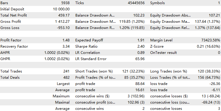
Now, let's run the backtest on the EA with the LSTM implementation, using a threshold of 30, as an ADX of 30 is widely recognized as indicating strong trend strength.

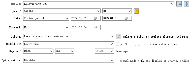
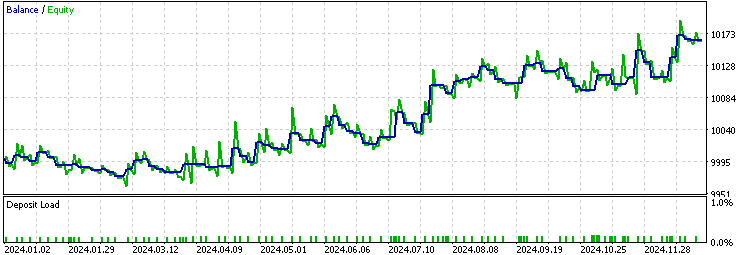
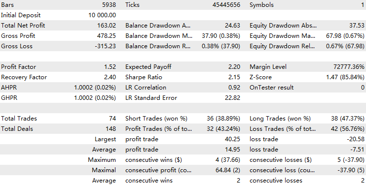
By comparing the two results, we observe that the LSTM implementation filtered out about 70% of the original trades and improved the profit factor from 1.48 to 1.52. It also exhibited a higher LR correlation than the baseline, suggesting that it contributed to more stable overall performance.

When backtesting machine learning models, it is important to recognize that the model's internal parameters are key determinants, unlike simpler strategies where parameters have less impact. As a result, different training data can lead to very different parameter outcomes. Additionally, training on the entire historical dataset at once is not ideal, as it would result in too many samples, most of which would lack timeliness. For this reason, I recommend using the sliding window method for backtesting in such cases. If we have limited samples throughout the entire backtest history, as discussed in my previous article on the CatBoost model, an expanding window backtest is more suitable.

Here are the demonstration images:

Sliding Window Backtest involves using a fixed-size window of historical data that moves forward in time. As new data points are added, the oldest data points are dropped, maintaining a constant data window size for testing the strategy's performance over different periods.

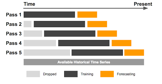
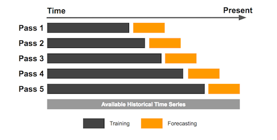
Expanding Window Backtest starts with an initial fixed-size data window, but as new data points become available, the window expands to include the new data, testing the strategy on an increasingly larger dataset over time.

To perform the sliding backtest, we simply repeat the process outlined in this article and merge the results into a single dataset. Here is the sliding backtest performance from January 1, 2015, to January 1, 2025:

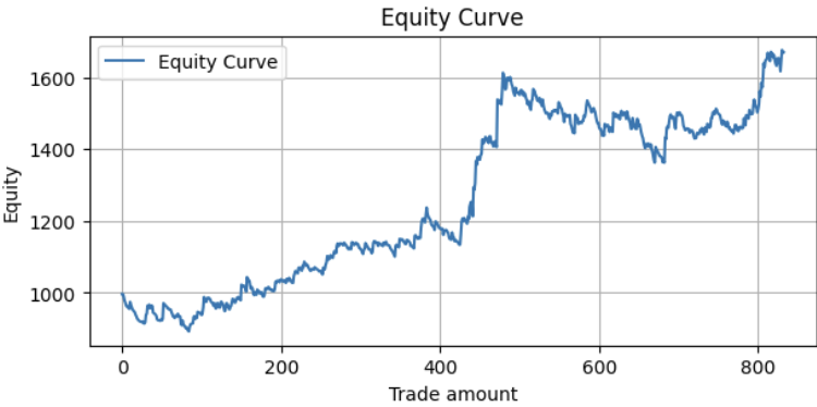
Metrics:

Profit Factor: 1.24
Maximum Drawdown: -250.56
Average Win: 12.02
Average Loss: -5.20
Win Rate: 34.81%

The result is impressive, with room for further improvement.

Reflection

The performance of the EA directly correlates with the predictability exhibited by the model. To improve your EA, there are a few key factors to consider:

1. The edge of your backbone strategy: Ultimately, the majority of your original signals need to have an edge to justify further filtering.
2. The data used: Market inefficiencies are revealed by analyzing the feature importance of each input and identifying lesser-known features that could provide an advantage.
3. The model you use to train: Think about whether it's a classification or regression problem you are trying to solve. And choosing the right training parameters is crucial, too.
4. The things you are trying to predict: Instead of directly predicting the outcome of a trade, focus on something indirectly related to the final result, as I demonstrate in this article.

Throughout my previous articles, I’ve experimented with various machine learning techniques that are accessible to retail traders. My goal is to inspire readers to adopt these ideas and develop their own innovative approaches, as creativity in this field is limitless. Machine learning isn't inherently complex or out of reach—it's a mindset. It’s about understanding the edge, constructing predictive models, and testing hypotheses rigorously. As you continue experimenting, this understanding will gradually become clearer.

Conclusion

In this article, we first introduced the motivation for using LSTM to predict trends, while explaining the concepts behind ADX and LSTM. Next, we fetched data from MetaTrader 5, processed it, and trained the model in Python. We then walked through the process of constructing the Expert Advisor and reviewing the backtest results. Finally, we introduced the concepts of sliding window backtesting and expanding window backtesting, and concluded the article with some reflective thoughts.

File Table

File Name	File Usage
FileCSV.mqh	The include file for storing data into CSV
LSTM_Demonstration.ipynb	The python file for training LSTM model
LSTM-TF-XAU.mq5	The trading EA with LSTM implementation
OHLC Getter.mq5	The EA for fetching data