MQL5 Wizard Techniques you should know (Part 60): Inference Learning (Wasserstein-VAE) with Moving Average and Stochastic Oscillator Patterns

Introduction

In examining the patterns generated from pairing the MA and stochastic oscillator, we have looked to machine learning as a means of systemizing our approach. There are mainly three methods of training networks in machine learning and these are supervised-learning, reinforcement-learning, and inference. By taking the view that each of these learning methods can be used at different stages of model/ network development, we have made the case that a model can be enriched by incorporating all of them.

Brief Recap

To do a brief recap, our earlier supervision-learning article, involved modelling features to states. Features are the indicator patterns of both the MA and Stochastic Oscillator. States are forecast changes in price that lag our indicator patterns, and are predicted by our model/ network. The simple diagram below helps illustrates this.

 

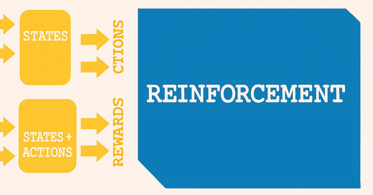
The use of the name ‘states’ to forecast price changes is fortuitous because from supervised-learning we move to reinforcement-learning. As it is established within reinforcement-learning, states are a key starting point to the training process, that much resembles the diagram below.

There are a number of variations in reinforcement-learning depending on the algorithm used but for most, in principle, they use two networks. The first being a policy that is shown as the upper of the two networks in the diagram above and the other being the value network which is represented as the lower.

Reinforcement can be a sole training method for a model or system, but we argued in the last article that it could be used more on live deployed models. When this is done, the exploration/ exploitation balance would be more relevant in ensuring an already trained model adapts to changing market environments. But even more than that, we saw how decisions to go long or short can be processed further in selecting the kind of action necessary for a forecast state.

Inference

This then leads us to inference, or what is also referred to as unsupervised-learning. What is the objective of inference? When I first started thinking about this, I was of the view that it allowed us to take trained networks/models for a given situation and, with some minor adjustments and tuning, apply it in a different setting. For traders, this translates to training a model for EUR USD and then, with slight adjustments, transferring that knowledge to say EUR JPY. However, as most traders will testify, even developing a non-arbitrage Expert Advisor that can trade more than one symbol concurrently is a tenuous process with a problematic risk-reward profile.

And, on top of that, the compute cost of training different models across multiple currency pairs is no longer as prohibitive as it once was. This is thanks in large part to faster GPUs, and the prevalence of cloud infrastructure that brings this to so many users. This situation thus, on paper, should lead to the creation of many models. While storage costs are also declining, especially when one considers that large multimillion parameter models are now being stored like regular computer files, I think inference via encoders makes the case for this knowledge to be compressed and ‘more storable’.

Now, because the need for more or special storage is almost mute, given how cheap it is, one could easily dismiss this. This is particularly true if you consider that with a supervised-learning model already trained and a reinforcement-learning system in place to keep it abreast, what would inference bring to the table? Well, we argue that not all data is in continuous time series form. 

If one considers cases of old historical data that could be similar in some way to current or unfolding events, inference can help in mapping this while minimizing the white noise. By mapping, we are referring to the setup illustrated in the diagram below:

So with a situation where features for historical data are available we show below how with no-supervision (in this case linear-regression) we can infer the respective states-actions-rewards. This is all because we trained a Variational-Auto-Encoder model to pair features-states-actions-rewards (FSAR) to a hidden layer that we refer to as encodings. With datasets of FSAR and encodings, we thus fit a linear-regression model that then helps us in filling missing gaps within an FSAR dataset. This is the primary application we are going to explore in this article.

However, if one also takes a step back and looks at the supervised-learning process, and the reinforcement-learning process, it does become clear that as the time passes, there grows a need to more wholistically integrate the knowledge gathered. And while performing another supervised-learning stint over this longer period and then running reinforcement-learning can be an option, inference-learning should be a more scalable and wholistic alternative.

So, to wrap up our introduction, inference is the estimating of hidden variables from observed data. In Bayesian models, usually, inference is the process of calculating the posterior distribution of hidden variables when presented with visible-layer datasets. Mathematically, therefore, it can be formally defined as follows:

Where:

• z is the latent variable or encodings,
  
  
• x is the observed data, which in our case is FSAR,
  
  
• p(z∣x) is the posterior (what we want to learn) or the probability of observing z given that x has been seen,
  
  
• p(x∣z) is the likelihood or probability of seeing x when presented with z
  
  
• p(z) is the prior,
  
  
• p(x) is the evidence.

P(x) is often intractable or hard to compute.

Why is it hard? The denominator, p(x), involves integrating over all possible latent variables:

This is generally computationally intractable in high dimensions, i.e., as the latent variable increases in size.

How then can VAEs help? VAEs convert the problem of approximate inference into an optimization task. This is achieved with the introduction of an encoder/ inference-network and a decoder/ generative-network. The encoder answers the question to q(z|x) which is a learned approximation of the exterior; while the decoder network addresses p(x|z) which is a reconstruction of the data (in our case FSAR) from the latent code (encodings).

VAE’s key innovation though is instead of computing the posterior exactly, the VAE would optimize for the Evidence Lower Bound Optimization (ELBO). The ELBO is the objective function used to train VAEs by approximating the true data distribution while ensuring the model learns meaningful latent representations and less noise. Here is the key-intuition:

As already mentioned above, computing p(x) is very hard and intractable; however, proving p(x) and for that matter log p(x) is more than a given value is feasible and tractable. Since our goal is to maximize p(x), by maximizing or raising the lower bound, we end up also raising p(x). VAE learns to infer latent structure from the data and is trained end-to-end with gradient descent. It thus demonstrates both amortized inference and generative modeling in one framework.

Why is VAE core to Inference Philosophy? Because the VAE learns to perform inference via the encoder. This means that instead of solving the inference problem whenever there is a new set of data, a shared encoder is used. This is also referred to as amortized inference. This is an excellent tool for weighing the trade-off between fidelity & regularity, but also understanding in general how latent variables represent generative structure.

We are implementing the VAE for this article by exploring Wasserstein Distanceinstead of the traditional KL-divergence when comparing distributions. Reasons for this are mostly exploratory, as we could in future articles consider the KL-divergence. However, it has been argued that KL-divergence overly constrains the latent space, which in turn can lead to posterior collapse. Secondly, the Wasserstein distance, it is argued, is a more flexible metric for comparing distributions, particularly in situations where the distributions in questions have little to no overlap.

The core idea of Wasserstein distance is to measure the “cost” of transforming one probability distribution into another. That's why it's sometimes referred to as the Earth-Mover’s distance. It is captured by the following equation:

Where:

• P: True data distribution (e.g., Gaussian prior p(z)).

• Q: Approximate distribution (e.g., encoder’s output q(z∣x)).

• γ: A joint distribution (coupling) over P and Q.

• Γ(P,Q): Set of all possible couplings between P and Q.

• ∥x−y∥: Distance metric (e.g., Euclidean distance).

• inf: Infimum (greatest lower bound, i.e., the smallest possible transport cost).

Wasserstein therefore calculates the least amount of “work” required to move mass Q to match P. Wasserstein VAE is important because it produces sharper samples, has more expressive latent representations. It is generally thought to be more stable when training under certain conditions.

There are primarily two Common implementations of Wasserstein VAE. WVAE-MMD, and WVAE-GAN. The former utilizes Maximum-Mean-Discrepancy to compare p(z) and q(z). Its what we are going to use for this article. As a side note the later, WVAE-GAN, uses adversarial loss to align latent distributions. We may also look at this implementation in future articles. The Maximum-Mean-Discrepancy is captured by the following equation:

Where:

• P: True prior (e.g., p(z)=N(0,I)).

• Q: Encoder’s distribution (e.g., q(z∣x)).

• k(⋅,⋅): Kernel function (e.g., Gaussian RBF).

• x,x′: Two independent samples from P.

• y,y′: Two independent samples from Q.

MMD compares mean-embeddings of P and Q in a high-dimensional space (Reproducing Kernel Hilbert Space). The closer these means are too matching, the more similar the distributions are.

VAE Implementation

We these start off by implementing our models/ networks in Python, primarily because it is more expedient to train them here than in raw MQL5. There are workarounds in MQL5 that involve using OpenCL that can reduce the performance gap, however we are yet to look at these, within these series. We implement a Wasserstein VAE class as follows in Python:

class WassersteinVAEUnsupervised(nn.Module):
    def __init__(self, feature_dim, encoding_dim, k_neighbors=5):
        super().__init__()
        self.encoding_dim = encoding_dim
        self.k_neighbors = k_neighbors
        
        # Feature encoder
        self.feature_encoder = nn.Sequential(
            nn.Linear(feature_dim, 256),
            nn.ReLU(),
            nn.Linear(256, 128),
            nn.ReLU(),
            nn.Linear(128, encoding_dim * 2)  # mean and logvar
        )
        
        # Buffer for storing training references
        self.register_buffer('ref_encoding', torch.zeros(1, encoding_dim))
        self.register_buffer('ref_states', torch.zeros(1, 1))
        self.register_buffer('ref_actions', torch.zeros(1, 1))
        self.register_buffer('ref_rewards', torch.zeros(1, 1))
        self._references_loaded = False
    
    def encode(self, features):
        h = self.feature_encoder(features)
        z_mean, z_logvar = torch.chunk(h, 2, dim=1)
        return z_mean, z_logvar
    
    def reparameterize(self, mean, logvar):
        std = torch.exp(0.5 * logvar)
        eps = torch.randn_like(std)
        return mean + eps * std
    
    def update_references(self, encoding_vectors, states, actions, rewards):
        """Store reference data for unsupervised prediction"""
        self.ref_encoding = encoding_vectors.detach().clone()
        self.ref_states = states.detach().clone().unsqueeze(-1)
        self.ref_actions = actions.detach().clone().unsqueeze(-1)
        self.ref_rewards = rewards.detach().clone().unsqueeze(-1)
        self._references_loaded = True
    
    def knn_predict(self, z, ref_values):
        # z shape: [batch_size, encoding_dim]
        # ref_values shape: [ref_size, 1] or [ref_size]
        
        # Ensure ref_values is properly shaped
        ref_values = ref_values.view(-1)  # Flatten to [ref_size]
        
        # Calculate distances between z and reference encodings
        distances = torch.cdist(z, self.ref_encoding)  # [batch_size, ref_size]
        
        # Get top-k nearest neighbors
        _, indices = torch.topk(distances, k=self.k_neighbors, largest=False)  # [batch_size, k]
        
        # Gather corresponding reference values
        neighbor_values = torch.gather(
            ref_values.unsqueeze(0).expand(indices.size(0), -1),  # [batch_size, ref_size]
            1,
            indices
        )  # [batch_size, k]
        
        # Average the nearest values
        predictions = neighbor_values.mean(dim=1, keepdim=True)  # [batch_size, 1]
        
        return predictions
    
    def gaussian_predict(self, z, ref_values):
        # Input validation
        assert z.dim() == 2, "z must be 2D [batch, encoding]"
        assert ref_values.dim() == 2, "ref_values must be 2D"
        
        # Calculate distances (Euclidean)
        distances = torch.cdist(z, self.ref_encoding)  # [batch, ref_size]
        
        # Convert to similarities (Gaussian weights)
        weights = torch.softmax(-distances, dim=1)  # [batch, ref_size]
        
        # Prepare reference values
        ref_values = ref_values.squeeze(-1) if ref_values.size(1) == 1 else ref_values
        ref_values = ref_values.unsqueeze(0) if ref_values.dim() == 1 else ref_values
        
        # Ensure proper shapes
        ref_values = ref_values.view(-1, 1)  # Force [792, 1] shape
        
        # Calculate distances
        distances = torch.cdist(z, self.ref_encoding)  # [batch_size, 792]
        
        # Convert to weights
        weights = torch.softmax(-distances, dim=1)  # [batch_size, 792]
        
        # Matrix multiplication Weighted combination
        predictions = torch.matmul(weights, ref_values)  # [batch, 1]
        
        return predictions.unsqueeze(-1) if predictions.dim() == 1 else predictions
    
    def linear_predict(self, z, ref_values):
        """Linear regression prediction using normal equations"""
        # Add bias term
        X = torch.cat([self.ref_encoding, torch.ones_like(self.ref_encoding[:, :1])], dim=1)
        y = ref_values
        
        # Compute closed-form solution
        XtX = torch.matmul(X.T, X)
        Xty = torch.matmul(X.T, y)
        theta = torch.linalg.solve(XtX, Xty)
        
        # Predict with new z values
        X_new = torch.cat([z, torch.ones_like(z[:, :1])], dim=1)
        return torch.matmul(X_new, theta)

    def predict_from_encoding(self, z):
        if not self._references_loaded:
            raise RuntimeError("Reference data not loaded")
            
        # Validate reference shapes
        self.ref_states = self.ref_states.view(-1, 1)
        self.ref_actions = self.ref_actions.view(-1, 1)
        self.ref_rewards = self.ref_rewards.view(-1, 1)
        
        states = self.knn_predict(z, self.ref_states)
        actions = self.gaussian_predict(z, self.ref_actions)
        rewards = self.linear_predict(z, self.ref_rewards)
        
        return states, actions, rewards
    
    def forward(self, features, states=None, actions=None, rewards=None):
        z_mean, z_logvar = self.encode(features)
        z = self.reparameterize(z_mean, z_logvar)
        
        if states is not None and actions is not None and rewards is not None:
            return {
                'z': z,
                'z_mean': z_mean,
                'z_logvar': z_logvar
            }
        else:
            pred_states, pred_actions, pred_rewards = self.predict_from_encoding(z)
            return {
                'states': pred_states,
                'actions': pred_actions,
                'rewards': pred_rewards
            }

Our Wasserstein VAE implementation above consists primarily of four things. A feature encoder, reference buffer, prediction methods, and a dual-mode forward pass. The feature encoder is a 3-layer MLP whose role is to compress inputs to latent space parameters (of z, z-mean & z-logvar). The reference buffers store pre-trained model inputs of features, states, actions, and rewards together with their respective encodings. The prediction methods listed are for forecasting states, actions, and rewards for an incomplete data set that is presented with only features. These methods are K-NN, Gaussian-Weighting, Linear-Regression. They work within the latent space by mapping encodings to the missing data points of states-actions-rewards. The dual-mode forward pass handles both training and inference.

Key functional components are the encoding process, reference system, prediction mechanisms, and inference flow. In the encoding process, input features-states-actions-rewards pass through the encoder network. The output splits these inputs into an ‘encoding’ of z, z-mean, and z-log-var. Also in the process, reparametrization trick allows us to have differentiable sampling. The reference system stores the ‘frozen’ outputs with their respective FSAR input pairings. It requires explicit initialization via the update_references() function.

The 3 prediction mechanisms are targeted at forecasting states, actions, or rewards. Our model works with the basis that features are always available as part of the FSAR data set, however there are times when only the SAR (states-actions-rewards) could be missing. KNN clustering maps states, Gaussian Process Regression maps actions and Linear Regression maps rewards. The inference flow therefore encodes our input features to the latent space, selects the prediction method for each input type based on the pairings just mentioned, and then returns the respective state/ action/ reward estimates.

A few improvements could be made to our approach above, though. These can broadly fall in 3 buckets. Architectural enhancements, training improvements, or just more robustness. The architecture improvements could include: adding spectral normalization to enforce Lipschitz continuity; implementing learnable temperature for the Gaussian Process weighting; including reference memory management (FIFO/ Pruning); and adding Monte-Carlo sampling for uncertainty estimation. The training process can also be improved by introducing a gradient penalty for Wasserstein constraints; adding latent space regularization (MMD/ coverage terms); implementing adaptive prediction method selection; and adding ensemble weighting of prediction methods.

Robustness improvements are a little ambiguous, however endeavors could be made with: out-of-distribution detection capability; reference quality scoring system; dynamic neighborhood size adjustment; and input-dependent noise scaling.

MMD-Loss Implementation

The form of the Wasserstein VAE we are implementing is the MMD-Loss and its two loss functions that we use for the VAE are presented below:

def mmd_loss(y_true, y_pred, kernel_mul=2.0, kernel_num=5):
    """
    MMD loss using Gaussian RBF kernel.
    Args:
        y_true: Ground truth samples (shape: [batch_size, dim])
        y_pred: Predicted samples (shape: [batch_size, dim])
        kernel_mul: Multiplier for kernel bandwidths
        kernel_num: Number of kernels to use
    Returns:
        MMD loss (scalar)
    """
    batch_size = y_true.size(0)
    
    # Combine real and predicted samples
    xx = y_true
    yy = y_pred
    xy = torch.cat([xx, yy], dim=0)
    
    # Compute pairwise distances
    distances = torch.cdist(xy, xy, p=2)
    
    # Compute MMD using multiple RBF kernels
    loss = 0.0
    for sigma in [kernel_mul ** k for k in range(-kernel_num, kernel_num + 1)]:
        if sigma == 0:
            continue
        kernel_val = torch.exp(-distances ** 2 / (2 * sigma ** 2))
        k_xx = kernel_val[:batch_size, :batch_size]
        k_yy = kernel_val[batch_size:, batch_size:]
        k_xy = kernel_val[:batch_size, batch_size:]
        
        # MMD formula: E[k(x,x)] + E[k(y,y)] - 2*E[k(x,y)]
        loss += (k_xx.mean() + k_yy.mean() - 2 * k_xy.mean())
    
    return loss / (2 * kernel_num)

def compute_loss(predictions, batch):
    # Ensure shapes match (squeeze if needed)
    pred_states = predictions['states'].squeeze(-1)  # [B, 1] → [B]
    pred_actions = predictions['actions'].squeeze(-1)
    pred_rewards = predictions['rewards'].squeeze(-1)
    
    # MMD Loss (distributional matching)
    mmd_state = mmd_loss(batch['states'], pred_states)
    mmd_action = mmd_loss(batch['actions'], pred_actions)
    mmd_reward = mmd_loss(batch['rewards'], pred_rewards)
    
    # Combine losses (adjust weights as needed)
    total_loss = mmd_state + mmd_action + mmd_reward
    
    return {
        'loss': total_loss,
        'mmd_state': mmd_state,
        'mmd_action': mmd_action,
        'mmd_reward': mmd_reward
    }

The MMD-Loss function input parameters are y_true and y_pred. They represent a comparison of the ground-truth and generated samples. Their dimension-alignment is important in order to be able to compute a comparison. The kernel_mul/ kernel_num inputs control the RBF kernel bandwidths, and therefore affect sensitivity to various scales of the distribution differences.

The sample combination, xy, brings together real and generated samples to compute all pairwise distances in one operation. This is memory efficient and ensures consistent distance computations. The distance's computation uses p=2 (Euclidean distance) which is standard for MMD. This choice directly influences the sensitivity to distributional differences. The ‘cdist’ operation is the meat and potatoes, mathematically, since MMD relies on pairwise comparisons.

The multi-kernel approach uses geometrically spaced bandwidths (kernel_mul^k) to get a sense of the multiscale distribution characteristics. It avoids the sigma=0 scenario which brings zero-divides. Each kernel contributes equally to the final loss through averaging. The MMD calculation uses the core formula (k_xx + k_yy - 2k_xy) that quantifies discrepancies between distributions. Mean operations provide expectation estimates from finite samples, and the normalization by kernel count makes the loss scale consistent across different configurations.

Improvements to this MMD could be made with kernel selection, where: adding adaptive bandwidth selection can be implemented based on sample statistics; experiments with non-RBF kernels can be performed to establish which kernels are best suited for which data types; implementing of automatic relevance determination can be done for the bandwidths. Numerical stability can also be introduced by: adding small epsilon to the denominator for stability; implementing log-domain computations for very small kernel values; and clipping extreme distance values to prevent overflow. Other measures can cover computation efficiency, and VAE integration. 

There is a lot of other code that we have to use in running this inference that we are not explicitly highlighting here. Noteworthy though is that the generation of FASR input data comes from running code from the earlier 2 articles on the MA and Stochastic Oscillator. The supervised-learning article gives us the features and states components of our VAE input, while the reinforcement-learning article code gives us the actions and rewards.

Linear-Regression Implementation

In order to use our inference model, we rely solely on the regression functions that map from the latent layer to the missing inputs and not the VAE network. This contrasts what we have been doing in the past articles, where we had to export the network we had trained as an ONNX file. 

The reason this is the case is we are interested in completing the input dataset to a VAE that we have trained.

Going forward, we have only features data. So the question becomes based what are the states, actions, and rewards for these features. In order to answer this question, we at initialization of our Expert Advisor we need to train a linear regression model with datasets of pairs for features-encodings, states-encodings, actions-encodings, and rewards-encodings. With our Linear Regression model trained (or fitted), for any new features data point of new data, we would map it to an encoding, and then use this encoding within the same model to map back to states, actions, and rewards.

This fitting process of getting the encodings connections uses unsupervised learning. Our Linear Regression is implemented as follows in MQL5:

//+------------------------------------------------------------------+
// Linear Regressor (unchanged from previous implementation)         |
//+------------------------------------------------------------------+
class LinearRegressor
{
private:
   vector m_coefficients;
   double m_intercept;

   matrix m_coefficients_2d;
   vector m_intercept_2d;

public:
   void Fit(const matrix &X, const vector &y)
   {  int n = (int)X.Rows();
      int p = (int)X.Cols();
      matrix X_with_bias(n, p + 1);
      for(int i = 0; i < n; i++)
      {  for(int j = 0; j < p; j++)
            X_with_bias[i][j] = X[i][j];
         X_with_bias[i][p] = 1.0;
      }
      matrix Xt = X_with_bias.Transpose();
      matrix XtX = Xt.MatMul(X_with_bias);
      matrix XtX_inv = XtX.Inv();
      vector y_col = y;
      y_col.Resize(n, 1);
      vector beta = XtX_inv.MatMul(Xt.MatMul(y_col));
      m_coefficients = beta;
      m_coefficients.Resize(p);
      m_intercept = beta[p];
   }

   void Fit2d(const matrix &X, const matrix &Y)
   {  int n = (int)X.Rows();    // Number of samples
      int p = (int)X.Cols();    // Number of input features
      int k = (int)Y.Cols();    // Number of output encodings
      // Add bias term (column of 1s) to X
      matrix X_with_bias(n, p + 1);
      for(int i = 0; i < n; i++)
      {  for(int j = 0; j < p; j++)
            X_with_bias[i][j] = X[i][j];
         X_with_bias[i][p] = 1.0;
      }
      // Calculate coefficients using normal equation: (X'X)^-1 X'Y
      matrix Xt = X_with_bias.Transpose();
      matrix XtX = Xt.MatMul(X_with_bias);
      matrix XtX_inv = XtX.Inv();
      matrix beta = XtX_inv.MatMul(Xt.MatMul(Y));
      // Split coefficients and intercept
      m_coefficients_2d.Resize(p, k);  // Coefficients for each output encodings
      m_intercept_2d.Resize(k);        // Intercept for each input feature
      for(int j = 0; j < p; j++)
      {  for(int d = 0; d < k; d++)
         {  m_coefficients_2d[j][d] = beta[j][d];
         }
      }
      for(int d = 0; d < k; d++)
      {  m_intercept_2d[d] = beta[p][d];
      }
   }

   double Predict(const vector &x)
   {  return m_intercept + m_coefficients.Dot(x);
   }

   vector Predict2d(const vector &X) const
   {  int p = (int)X.Size();    // Number of input features
      int k = (int)m_intercept_2d.Size(); // Number of output encodings
      vector predictions(k);  // vector to store predictions
      for(int d = 0; d < k; d++)
      {  // Initialize with intercept for this output dimension
         predictions[d] = m_intercept_2d[d];
         // Add contribution from each feature
         for(int j = 0; j < p; j++)
         {  predictions[d] += m_coefficients_2d[j][d] * X[j];
         }
      }
      return predictions;
   }
};

The core structure maintains separate coefficient storage for 1D (for variables m_coefficients/m_intercept) and 2D (for variables m_coefficients_2d/m_intercept_2d). Matrix algebra is used for some efficiency in batch operations. It implements both single-output and multi-output regression variants. Its fitting methods use the Normal Equation by directly solving (X'X)^- 1X'y. It handles bias by adding a column of 1s to input features. 2D-Specialization by the class also handles multiple outputs simultaneously via matrix operations.

The prediction methods use a dot-product implementation, which serves as an efficient linear combination of inputs and weights. Dimension handling is properly processed for both single and multi-output scenarios, and memory management pre-allocates the result vector for efficiency. We use a pseudo Wasserstein VAE class to call and implement our state-actions-and rewards forecasts. This is coded in MQL5 as follows:

//+------------------------------------------------------------------+
// Wasserstein VAE Predictors Implementation (unchanged)             |
//+------------------------------------------------------------------+
class WassersteinVAEPredictors
{
private:
   LinearRegressor m_feature_predictor;
   LinearRegressor m_state_predictor;
   LinearRegressor m_action_predictor;
   LinearRegressor m_reward_predictor;
   bool m_predictors_trained;

public:
   WassersteinVAEPredictors() : m_predictors_trained(false) {}

   void FitPredictors(const matrix &features,
                      const vector &states,
                      const vector &actions,
                      const vector &rewards,
                      const matrix &encodings)
   {  m_feature_predictor.Fit2d(features, encodings);
      m_state_predictor.Fit(encodings, states);
      m_action_predictor.Fit(encodings, actions);
      m_reward_predictor.Fit(encodings, rewards);
      m_predictors_trained = true;
   }

   void PredictFromFeatures(const vector &y, vector &z)
   {  if(!m_predictors_trained)
      {  Print("Error: Predictors not trained yet");
         return;
      }
      z = m_feature_predictor.Predict2d(y);
   }

   void PredictFromEncodings(const vector &z, double &state, double &action, double &reward)
   {  if(!m_predictors_trained)
      {  Print("Error: Predictors not trained yet");
         return;
      }
      state = m_state_predictor.Predict(z);
      action = m_action_predictor.Predict(z);
      reward = m_reward_predictor.Predict(z);
   }
};

We also, within our custom signal class, now rely on an ‘Infer’ function to process our forecasts. This is as follows:

//+------------------------------------------------------------------+
//| Inference Learning Forward Pass.                                 |
//+------------------------------------------------------------------+
vector CSignal_WVAE::Infer(int Index, ENUM_POSITION_TYPE T)
{  vectorf _f = Get(Index, m_time.GetData(X()), m_close, m_ma, m_ma_lag, m_sto);
   vector _features;
   _features.Init(_f.Size());
   _features.Fill(0.0);
   for(int i = 0; i < int(_f.Size()); i++)
   {  _features[i] = _f[i];
   }
// Make a prediction
   vector _encodings;
   _encodings.Init(__ENCODINGS);
   _encodings.Fill(0.0);
   double _state = 0.0, _action = 0.0, _reward = 0.0;
   if(Index == 1)
   {  m_vae_1.PredictFromFeatures(_features, _encodings);
      m_vae_1.PredictFromEncodings(_encodings, _state, _action, _reward);
   }
   else if(Index == 2)
   {  m_vae_2.PredictFromFeatures(_features, _encodings);
      m_vae_2.PredictFromEncodings(_encodings, _state, _action, _reward);
   }
   else if(Index == 5)
   {  m_vae_5.PredictFromFeatures(_features, _encodings);
      m_vae_5.PredictFromEncodings(_encodings, _state, _action, _reward);
   }
   vector _inference;
   _inference.Init(3);
   _inference[0] = _state;
   _inference[1] = _action;
   _inference[2] = _reward;
   //
   if(T == POSITION_TYPE_BUY)
   {  if(_state > 0.5)
      {  _inference[0] -= 0.5;
         _inference[0] *= 2.0;
         if(_action < 0.0)
         {  _inference[0] = 0.0;
         }
      }
      else
      {  _inference[0] = 0.0;
      }
   }
   else if(T == POSITION_TYPE_SELL)
   {  if(_state < 0.5)
      {  _inference[0] -= 0.5;
         _inference[0] *= -2.0;
         if(_action > 0.0)
         {  _inference[0] = 0.0;
         }
      }
      else
      {  _inference[0] = 0.0;
      }
   }
   return(_inference);
}

Guides are here and here on how to assemble an Expert Advisor by the MQL5 wizard for new readers. From the last article, of the 10 patterns we started with, only patterns 1, 2, and 5 were able to forward walk. Therefore, our long condition and short condition functions for this Expert Advisor only process these three patterns. We are forecasting 3 values. States, actions and rewards. States are bound to the range 0 to 1. Actions are also bound to a similar range, while rewards are in the range -1 to +1. Anyone with some experience with training and using neural networks would know that the test or deploy outputs of neural networks after training with targets that respect set bound limits, do not always fall within the expected bound limits. Some form of post forward run normalization is often required.

We do not perform any normalizations here, but simply bring this to the attention of the reader as something he should keep in mind when rolling out a trained network into production. We upload 2 years of daily price data for EUR USD to Python to train a VAE that provides us with dataset pairing of features-states-actions-rewards with encodings. This data set in turn is fitted to linear regression models that we then use to map out states, actions, and rewards when presented with features. Of this uploaded data, which is handled via Meta Trader 5 Python’s module, 80% of it is used in training, with 20% left for testing.

The data period is from 2023.01.01 to 2025.01.01. So a forward walk would be approximately the 5 months prior to 2025.01.01. We perform tests for a slightly longer period, the 6-months before i.e. 2024.07.01 to 2025.01.01 and are presented with the following reports:

For pattern 1:

For pattern 2:

For pattern 5:

It appears only patterns 1 and 5 are able to capitalize on inference based on a short 2-year train/ test window.

Conclusion

We wrap up our look at Moving Average and Stochastic Oscillator Patterns that are harnessed with machine learning by exploring the inference-learning use case. We have presented a possible implementation path for inference-learning based on the argument that once supervised-learning is done and reinforcement-learning is also rolled out on a live test environment; there remains a need for a more wholistic approach to gather and ‘store’ all the knowledge from supervised learning and well as reinforcement-learning. I believe that inference learning is poised and suited to playing this role, especially since its learning method is not duplicitous to what we have already used with supervised-learning and reinforcement-learning.

Name	Description
wz_60.mq5	Wizard Assembled Expert Advisor included for header to show necessary assembly files
SignalWZ_60.mqh	Signal Class file
60_vae_1.onnx	VAE ONNX model for pattern 1, not necessary for Expert Advisor.
60_vae_2.onnx	VAE ONNX model for pattern 2, ditto
60_vae_5.onnx	VAE ONNX model for pattern 5, ditto