Tuning LLMs with Your Own Personalized Data and Integrating into EA (Part 5): Develop and Test Trading Strategy with LLMs(I)-Fine-tuning

Table of contents

• Table of contents
• Introduction
• Fine-tuning of Large Language Models
• Formulation of Trading Strategy
• Creation of Dataset
• Fine-tuning the Model
• Testing
• Conclusion
• References

Introduction

In our previous article, we introduced how to use GPU acceleration to train large language models, but we did not use it to formulate trading strategies or perform backtesting. However, the ultimate goal of training our model is to use it and let it serve us. So, starting from this article, we will step by step use the trained language model to formulate trading strategies and test our strategies on foreign exchange currency pairs. Of course, this is not a simple process. It requires us to adopt corresponding technical means to achieve this process. So let's implement it step by step.

The whole process may take several articles to complete.

• The first step is to formulate a trading strategy; 
• The second step is to create a dataset according to the strategy and fine-tune the model (or train the model), so that the input and output of the large language model conform to our formulated trading strategy. There are many different methods to achieve this process, and I will provide as many examples as possible;
• The third step is the inference of the model and the fusion of output with the trading strategy and create EA according to our trading strategy. Of course, we still have some work to do in the inference phase of the model (choosing the appropriate inference framework and optimization methods: e.g. flash-attention, model quantization, speedup etc.); 
• The fourth step is to use historical backtesting to test our EA on the client side. 

Seeing this, some friends may wonder, I have already trained a model with my own data, why do I need to fine-tune it? The answer to this question will be given in this article.

Of course, the available methods are not limited to fine-tuning the large prophecy model. Other techniques can also be used, such as RAG technology (a technique that uses retrieval information to assist the large language model in generating content), and Agent technology (an intelligent body created by the inference of the large language model). If all these contents are completed in one article, the length of the article will be too long, and it will not be enough to read the rules and will appear chaotic, so we will discuss them in several parts. In this article, we mainly discuss our first and second steps, formulate trading strategies and we'll give an example of fine-tuning a large language model (GPT2).

Fine-tuning of Large Language Models

Before we start, we must first understand this fine-tuning. Some friends may have doubts: We already trained a model in the previous few articles, why do we need to fine-tune it? Why not use the trained model directly? To understand this question, we must first notice the difference between large language models and traditional neural network models: At this stage, large language models are basically based on the transformer architecture, which includes complex attention mechanisms. The model is complex and has a large number of parameters, so when training large language models, it generally requires a large amount of data for training, as well as high-performance computer hardware support, and the training time is generally tens of hours to several days or even tens of days. So, for individual developers, it is relatively difficult to train a language model from scratch (of course, if you have a gold mine at home, it’s another story).

At this time, using our own dataset to fine-tune the already trained large language model provides us with more choices. And the large language model that has been trained with a large amount of data on large-scale cluster computing has better compatibility and generalization ability. This does not mean that the model trained directly with specific data is not good enough. As long as the data volume and quality are good enough and large enough, and the hardware equipment is strong enough you can completely use your own dataset to train a model from scratch and the effect may be better.

This just means that fine-tuning gives us more choices. So, the mainstream paradigm of large language models is to pre-train language model training on a large amount of general data, and then fine-tune for specific downstream tasks to achieve the purpose of domain adaptation. The fine-tuning mentioned here is essentially the same as the transfer learning or fine-tuning of traditional neural networks, but there are also very considerable differences. The following specifically introduces the commonly used fine-tuning methods in large language models.

Fine-tuning large models can be divided into supervised learning fine-tuning methods, unsupervised learning fine-tuning methods, and reinforcement learning fine-tuning methods:

• Supervised learning fine-tuning method: This is the most common way, that is, to train the model using labeled data. For example, you can collect some dialogue question and answer datasets. In this process, set the target output and input as a pair of paired examples to optimize the model.
• Unsupervised learning fine-tuning method: When there is not enough marked text, the large language model can continue to pre-train on a large amount of unmarked text, which helps the model to better understand the language structure.
• Reinforcement learning fine-tuning method: Like traditional reinforcement learning, first build a text quality comparison model (equivalent to a Critor) as a reward model, and rank the quality of multiple different outputs given by the pre-training model for the same prompt word. At the same time, this reward model can use a binary classification model to judge the pros and cons between the two input results. Then, according to the given prompt word sample data, use the reward model to give the quality evaluation of the user prompt word completion result of the pre-training model, and get better results with the language model target. Reinforcement learning fine-tuning will make the result text generated by LLM based on the pre-training model get better results. Commonly used reinforcement learning methods include DPO, ORPO, PPO, etc.

Fine-tuning large models specifically commonly used methods are mainly divided into two categories, Model-Tuning and Prompt-Tuning:

1. Full parameter fine-tuning

The most direct way is to fine-tune the entire large language model, which means that all parameters will be updated to adapt to the new dataset. This method is also called inefficient fine-tuning, because as the parameter volume of the current large language model is getting larger and larger, the required hardware resources are exponentially increasing. To give an example: For example, to fine-tune a large language model with a parameter scale of 8B, it may require 2 80G video memories or a total of about 160G multi-card acceleration training. This hardware investment is believed to discourage most ordinary developers.

2. Adapter-Tuning

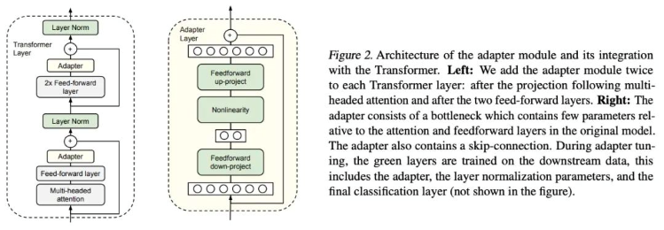
Adapter-Tuning is a PEFT fine-tuning method for BERT proposed by Google researchers for the first time, and it also kicked off the prelude to PEFT research. When facing a specific downstream task, if Full-finetuning (that is all parameters of the pre-training model are fine-tuned), it is too inefficient; and if the fixed pre-training model is used, only a few layers of parameters close to the downstream task are fine-tuned, and it is difficult to achieve better effect. So, they designed the Adapter structure, embedded it in the transformer structure, and during training, they fixed the parameters of the original pre-training model and only fine-tuned the newly added Adapter structure. At the same time, in order to ensure the efficiency of training (that is, to introduce as few more parameters as possible), they designed the Adapter as such a structure: first, a down-project layer maps high-dimensional features to low-dimensional features, and then passes a non-linear layer. After that, use an up-project structure to map low-dimensional features back to the original high-dimensional features. At the same time, a skip-connection structure is also designed to ensure that it can degrade to identity in the worst case.

Paper: "Parameter-Efficient Transfer Learning for NLP"(https://arxiv.org/pdf/1902.00751)

Code: https://github.com/google-research/adapter-bert

3. Parameter-Efficient Prompt-Tuning

Parameter-Efficient Prompt-Tuning is an efficient and practical model fine-tuning method. By adding continuous task-related embedding vectors before input for training, it can reduce the amount of computation and parameters and speed up the training process. At the same time, only a small amount of data is needed for effective fine-tuning, reducing the dependence on a large amount of labeled data. In addition, different Prompts can be customized for different tasks, which has strong task adaptability. In practical applications, Parameter-Efficient Prompt Tuning can help us quickly adapt to various task needs and improve the performance of the model. To implement Parameter-Efficient Prompt Tuning, we generally need the following steps:

• Define task-related embedding vectors-Define continuous task-related embedding vectors according to task needs. These vectors can be manually designed, or they can be automatically learned through other methods.
• Modify the input prefix: Add the defined embedding vector as a prefix before the input data. These prefixes will be passed to the model for training together with the original input.
• Fine-tune the model: Use the input data with the prefix for fine-tuning. In this process, only the parameters of the prefix part will be updated, and the parameters of the original pre-training model will remain unchanged.
• Evaluation and optimization: Evaluate the performance of the model on the validation set and make optimization adjustments. Through continuous iteration and optimization, we can get a fine-tuned model suitable for specific tasks.

Paper: “The Power of Scale for Parameter-Efficient Prompt Tuning Official” (https://arxiv.org/pdf/2104.08691.pdf)

Code: https://github.com/google-research/prompt-tuning

4. Prefix-Tuning

The Prefix-Tuning method proposes to add a continuous task-related embedding vector (continuous task-specific vectors) to each input for training. Prefix-Tuning is still a fixed pre-training parameter, but in addition to adding one or more embeddings for each task, it uses a multi-layer perceptron to encode the prefix (note that the multi-layer perceptron is the prefix encoder), and no longer continues to input LLM like prompt-tuning.

Here, continuous (continuous) is relative to the discrete (discrete) of manually defined text prompt tokens. For example, a manually defined prompt token array is [‘The’, ‘movie’, ‘is’, ‘[MASK]’], if the token there is replaced with an embedding vector as input, the embedding is a continuous (continuous) expression. When retraining the downstream task, fix all parameters of the original large model, and only retrain the prefix vector (prefix embedding) related to the downstream task. For self-regressive LM models (such as GPT-2 used in our current example), a prefix will be added before the original prompt (z = [PREFIX; x; y]); For the encoder+decoder LM model (such as BART), a prefix will be added to the input of the encoder and decoder respectively (z = [PREFIX; x; PREFIX’; y],).

Paper: “Prefix-Tuning: Optimizing Continuous Prompts for Generation, P-Tuning v2: Prompt Tuning Can Be Comparable to Fine-tuning Universally Across Scales and Tasks”(https://aclanthology.org/2021.acl-long.353)

Code: https://github.com/XiangLi1999/PrefixTuning

5. P-Tuning and P-Tuning V2

P-Tuning can significantly improve the performance of language models in multi-task and low-resource environments. It enhances input features by introducing a small-scale, easy-to-compute front-end subnetwork, thereby improving the performance of the base model. P-tuning still fixes LLM parameters, uses a multi-layer perceptron and LSTM to encode the prompt, and after encoding, it is normally input to LLM after concatenating with other vectors. Note that after training, only the vector after the prompt encoding is retained, and the encoder is no longer retained. This method can not only improve the accuracy and robustness of the model in various tasks, but also significantly reduce the amount of data and computational cost required during fine-tuning. The problem with p-tuning is that it performs poorly on small parameter models, so there is a V2 version, similar to LoRA, new parameters are embedded in each layer (referred to as Deep FT).

Specifically, P-Tuning v2 is an upgraded version based on P-Tuning. The main improvement is the adoption of a more efficient pruning method, which can further reduce the parameter volume of model fine-tuning. Strictly speaking, P-tuning V2 is not a brand-new method, it is an optimized version of Deep Prompt Tuning (Li and Liang,2021; Qin and Eisner,2021).

P-tuning v2 is designed for generation and knowledge exploration, but one of the most important improvements is to apply continuous prompts to each layer of the pre-training model, not just the input layer. This method only needs to fine-tune 0.1%-3% of the parameters, and it can be on par with Model Fine-Tuning, which shows its power!

P-Tuning paper: “GPT Understands, Too” (https://arxiv.org/pdf/2103.10385).

6. LoRA

The LoRA method first freezes the parameters of the pre-training model and adds additional parameters of dropout+Linear+Conv1d in each layer of the decoder. In fact, fundamentally speaking, LoRA cannot achieve the performance of full parameter fine-tuning. According to experiments, full parameter fine-tuning is much better than the LoRA method, but in low-resource situations, LoRA becomes a better choice. LoRA allows us to indirectly train some dense layers in the neural network by optimizing the rank decomposition matrix of the changes in the dense layer during adaptation, while keeping the pre-training weights frozen.

Features of LoRA:

• A well-pretrained model can be shared, used to build many small LoRA modules for different tasks. We can freeze the shared model, and effectively switch tasks by replacing the matrices A and B in Figure 1, thereby greatly reducing storage requirements and task switching overhead.
• LoRA makes training more efficient. When using adaptive optimizers, the hardware threshold is reduced by 3 times because we do not need to calculate gradients or maintain the optimizer status of most parameters. On the contrary, we only optimize the injected, much smaller low-rank matrix.
• Our simple linear design allows us to merge the trainable matrix with the frozen weights during deployment, and does not introduce inference delay in structure compared with the fully fine-tuned model.
• LoRA is irrelevant to many previous methods and can be combined with many methods.

Paper: “LORA: LOW-RANK ADAPTATION OF LARGE LANGUAGE MODELS” (https://arxiv.org/pdf/2106.09685.pdf).

Code: https://github.com/microsoft/LoRA.

7. AdaLoRA

There are many ways to decide which LoRA parameters are more important than others, and AdaLoRA is one of them, and the authors of AdaLoRA recommend considering the singular value of the LoRA matrix as an indicator of its importance.

An important difference from the LoRA-drop above is that the adapters in the middle layer of LoRA-drop are either fully trained or not trained at all. AdaLoRA can decide that different adapters have different ranks (in the original LoRA method, all adapters have the same rank).

AdaLoRA has a total of the same number of parameters compared to standard LoRA of the same rank, but the distribution of these parameters is different. In LoRA, the rank of all matrices is the same, while in AdaLoRA, some matrices have a higher rank and some matrices have a lower rank, so the final total number of parameters is the same. Experiments have shown that AdaLoRA produces better results than standard LoRA methods, which indicates that there is a better distribution of trainable parameters on the parts of the model, which is particularly important for a given task, and the layers closer to the end of the model provide a higher rank, indicating that adapting to these is more important.

AdaLoRA decomposes the weight matrix into an incremental matrix through singular value decomposition, and dynamically adjusts the size of the singular values in each incremental matrix, so that only those parameters that contribute more or are necessary to the model performance are updated during the fine-tuning process, to improve the model performance and parameter efficiency.

Paper: “ADALORA: ADAPTIVE BUDGET ALLOCATION FOR PARAMETER-EFFICIENT FINE-TUNING” (https://arxiv.org/pdf/2303.10512).

Code: https://github.com/QingruZhang/AdaLoRA.

8. QLoRA 

QLoRA backpropagates the gradient to the Low-Rank Adapter (LoRA) through a frozen 4-bit quantized pre-trained language model, which can greatly reduce memory usage and save computing resources while maintaining the performance of the complete 16-bit fine-tuning task.

Technical features of QLoRA:

• Backpropagation of gradients into low-order adapters (LoRAs) via a frozen, 4-bit quantized pre-trained language model.
• Introduce 4-bit NormalFloat (NF4), which is a theoretically optimal data type for quantizing information for normally distributed data, which can produce better empirical results than 4-bit integers and 4-bit floating-point.
• Apply double quantization, a method of quantifying quantification constants, saving about 0.37 bits per parameter on average.
• Use a paging optimizer with NVIDIA Unified Memory to avoid memory spikes during gradient checkpointing when processing small batches with long sequence lengths. Significantly reduced memory requirements, allowing fine-tuning of a 65B-parameter model on a single 48GB GPU without degrading runtime or predicting performance compared to a 16-bit fully fine-tuned benchmark.

Paper: “QLORA: Efficient Finetuning of Quantized LLMs” (https://arxiv.org/pdf/2305.14314.pdf).

Code: https://github.com/artidoro/qlora.

This article lists just a few commonly used representative methods, as well as some variants based on LoRA technology: LoRA+, VeRA, LoRA-fa, LoRA-drop, DoRA and Delta-LoRA, etc. This article will not introduce them one by one, interested you can consult the relevant literature.

Of course, there are some other prompt engineering that also meet our technical needs (such as RAG technology), in subsequent articles I will introduce them to you.

Next, we'll show you an example of fine-tuning GPT2 with full parameters.

Formulation of Trading Strategy

Regarding the trading strategy, we use a simple example to guide the fine-tuning of the large language model, temporarily not involving EA implementation (the specific implementation needs to wait until our complete large language model inference strategy is completed before we can reasonably create EA). First, get the latest 20 quotes’ closing prices of a certain period from a certain currency pair from the client, and define their average as A. Then use the large language model to predict the closing prices of the next 40 quotes of the same period, and define their average as B. Then judge whether to buy or sell next according to the predicted value:

• If the average value B of 40 predicted values is greater than the average value A of the current latest 20 closing prices, then buy.
• If the average value B of 40 predicted values is less than the average value A of the current latest 20 closing prices, then sell.
• If A and B are equal or very close, then do not operate.

Now we have completed the formulation of the trading strategy. This is a fairly simple trading strategy for demonstration, which may be idealized. You can also replace this strategy as you need, such as changing the input to dynamic, the total length of the prediction results 60 minus the length of the input. Or directly use other trading logics such as formulating rules based on wave strategy, or crocodile strategy, or turtle strategy, Of course, your model also needs to make corresponding adjustments. Next, we start to create a dataset according to the strategy and fine-tune the large language model.

Creation of Dataset

We have already made a dataset when we discussed training large language models earlier, which is the content contained in the “llm_data.csv” file. This dataset only contains the quotes of a currency pair on a 5M cycle, and has been processed accordingly, with a total of 2442 rows of data, each with 64 columns. For the specific processing process, please refer to the part of training large language models with CPU or GPU in this series of articles (The specific link is " Integrate Your Own LLM into EA (Part 3): Training Your Own LLM with CPU - MQL5 Articles "). Of course, you can also use the script provided in the article to re-customize the dataset or make your own excellent idea into a dataset (such as making the correlation between government fiscal data and exchange rate into a dataset, etc.). In short, this dataset can be in any form, not just numerical quotes. 

1. Preprocessing

First, we import the libraries we need:

import pandas as pd

from transformers import GPT2LMHeadModel, GPT2Tokenizer, GPT2Config

from transformers import TextDataset, DataCollatorForLanguageModeling

from transformers import Trainer, TrainingArguments

import torch

Read the data file:

df = pd.read_csv('llm_data.csv')

I updated this dataset, this dataset now contains 60 closing prices of a currency pair in a 5M cycle on each line, instead of the original 64, and the data is processed into text format:

sentences = [' '.join(map(str, prices)) for prices in df.iloc[:-10,1:].values]

This line of code mainly reads the entire Dataframe file, traverses its elements, and converts each line into a string, treating them as a sentence, each sentence contains 60 closing prices. That is, we convert it to: “0.6119 0.61197 0.61201…0.61196”, not: “0.6119” “0.61197”…“0.61196”. This is to let the language model remember the sequence length we set, for example, if we input 20 data, the model will complete the remaining 40 data for us, instead of outputting content that we cannot control.

There is also a special place in this line of code that needs to be explained, which is “df.iloc[:-10,1:].values”. The “:-10” means to take the beginning of the csv file to the last 10 lines, and we leave the remaining 10 lines for testing; “1:” is to remove the first column of each line, this column is the index value in the csv file, we don’t need it.

Next, we concatenate all the sequences into a dataset and save it as “train.txt”, so that we don’t need to process the csv file multiple times next time, just read the processed file directly.

with open('train.txt', 'w') as f:

    for sentence in sentences:

        f.write(sentence + '\n')

2. Load the data as a Dataset class

After our data preprocessing is over, we still need to use the tokenizer to further process the data and load it into the “Dataset” data format in pytorch. Now some commonly used classes are integrated in the Transformers library to directly complete this work. In the example in this article, you can directly use TextDataset to achieve this function, which is very simple, but we first need to use GPT2 to instantiate the tokenizer. If you have not loaded GPT2 before, then the first time you use it, the Transformers library will download the pre-training file from Huggingface, please ensure that the network is unblocked. Especially for friends who use docker or wsl, please make sure your network configuration is correct, otherwise the loading will fail.

tokenizer = GPT2Tokenizer.from_pretrained('gpt2')



train_dataset = TextDataset(tokenizer=tokenizer,

                            file_path="train.txt",     

                            block_size=60)

3. Load data for the language model

Here, we directly use the DataCollatorForLanguageModeling class in the Transformer library to instantiate the data, and we no longer need to do extra work.

data_collator = DataCollatorForLanguageModeling(tokenizer=tokenizer, mlm=False)

Next, let’s load the pre-trained model and fine-tune it.

Fine-tuning the Model

Once we have prepared our dataset for fine-tuning, we can begin the process of fine-tuning our large language model.

1. Loading the Pretrained Model

The first step in fine-tuning a model is to load the pretrained model. We have already loaded the tokenizer, so here we just need to load the model:

model = GPT2LMHeadModel.from_pretrained('gpt2')

Next, we need to set the training parameters. The Transformers library also provides us with a very convenient class to implement this function, without the need for additional configuration files:

training_args = TrainingArguments(output_dir="./gpt2_stock",     

                                  overwrite_output_dir=True,    

                                  num_train_epochs=3,     

                                  per_device_train_batch_size=32,   

                                  save_steps=10_000,    

                                  save_total_limit=2,

                                  load_best_model_at_end=True,

                                  )

2. Initializing Fine-tuning Parameters

When instantiating TrainingArguments, we used the following parameters:

• output_dir: The location to save prediction results and checkpoints. We defined the “gpt2_stock” folder in the current directory as the output path.
• overwrite_output_dir: Whether to overwrite the output file. We chose to overwrite.
• num_train_epochs: The number of training epochs. We chose 3 epochs.
• per_device_train_batch_size: The training batch size. We chose 32, which we introduced earlier, is best to be a power of 2.
• save_steps=10_000: The number of update steps before two checkpoint saves if save_strategy="steps". Should be an integer or a float in range [0,1). If smaller than 1, will be interpreted as a ratio of total training steps.
• save_total_limit: If a value is passed, will limit the total amount of checkpoints. Deletes the older checkpoints in output_dir.
• load_best_model_at_end: Whether to load the best model during the training process, rather than using the model weights at the last step of training.

There are many parameters that we did not set and used the default values because we are just an example, so we did not define this class in detail, for example:

• deepspeed: Whether to use Deepspeed to accelerate training.
• eval_steps: Number of update steps between two evaluations.
• dataloader_pin_memory: Whether you want to pin memory in data loaders or not.

You can see that this TrainingArguments class is very powerful, it almost includes most of the training parameters, it is very convenient to use, and it is highly recommended for readers to take a look at the official documentation.

3. Fine-tuning

Now let’s get back to our fine-tuning process, and now we can define our fine-tuning process. We have detailed the training process of the language model in the previous article. The fine-tuning process is not much different from the training process. I believe readers are already very familiar with it, so the example in this article no longer defines the fine-tuning process of the language model in detail, but directly uses the Trainer class provided in the Transformer library to implement it. Now we pass the model, training_args, data_collator, train_dataset that we have defined as parameters into the Trainer class to instantiate the Trainer:

trainer = Trainer(model=model,

                  args=training_args,

                  data_collator=data_collator,

                  train_dataset=train_dataset,)

The Trainer class also has other parameters that we did not set, such as the important callbacks: you can use callbacks to customize the behavior of the training loop, these callbacks can check the status of the training loop (for progress reporting, logging on TensorBoard or other ML platforms, etc.) and make decisions (such as early stopping, etc.). The reason why we did not set them in this article is because we are just an example and the parameter settings of the model in the fine-tuning process are relatively conservative. If you want your model to work better, please remember that this option should not be ignored. Call the tran() method of the instantiated Trainer class, and you can directly run the fine-tuning process:

trainer.train()

After the training is over, save the model, so that we can directly use the from_pretrained() method to load the fine-tuned model when we infer:

trainer.save_model("./gpt2_stock")

Next, let’s do an inference to check if the fine-tuning is effective:

prompt = ' '.join(map(str, df.iloc[:,1:20].values[-1])) 

generated = tokenizer.decode(model.generate(tokenizer.encode(prompt, return_tensors='pt').to("cuda"), 
		do_sample=True, 
		max_length=200)[0], 
		skip_special_tokens=True)

print(f"test the model:{generated}")

In this part of the code, “prompt = ' '.join(map(str, df.iloc[:,1:20].values[-1]))” converts the last line of our dataset into a string format. “tokenizer.encode(prompt, return_tensors=‘pt’)” This part of the code converts the input text (prompt) into a form that the model can understand, that is, it converts the text into a series of tokens. “return_tensors=‘pt’” indicates that the returned data type is a PyTorch tensor. “do_sample=True” indicates that random sampling is used in the generation process, and “max_length=200” limits the maximum length of the generated text. Now let’s take a look at the results of the entire code running: 

It can be seen that the fine-tuned pretrained model successfully output the results we wanted.

The complete code is as follows, the name of the script in the attachment is “Fin-tuning.py”:

import pandas as pd
from transformers import GPT2LMHeadModel, GPT2Tokenizer, GPT2Config
from transformers import TextDataset, DataCollatorForLanguageModeling
from transformers import Trainer, TrainingArguments
import torch

dvc='cuda' if torch.cuda.is_available() else 'cpu'

print(dvc)

df = pd.read_csv('llm_data.csv')

sentences = [' '.join(map(str, prices)) for prices in df.iloc[:-10,1:].values]
with open('train.txt', 'w') as f:
    for sentence in sentences:
        f.write(sentence + '\n')

tokenizer = GPT2Tokenizer.from_pretrained('gpt2')

train_dataset = TextDataset(tokenizer=tokenizer,
                            file_path="train.txt", 
                            block_size=60)

data_collator = DataCollatorForLanguageModeling(tokenizer=tokenizer, mlm=False)



model = GPT2LMHeadModel.from_pretrained('gpt2')

training_args = TrainingArguments(output_dir="./gpt2_stock",     
                                  overwrite_output_dir=True,    
                                  num_train_epochs=3,     
                                  per_device_train_batch_size=32,   
                                  save_steps=10_000,    
                                  save_total_limit=2,
                                  load_best_model_at_end=True,
                                  )

trainer = Trainer(model=model,
                  args=training_args,
                  data_collator=data_collator,
                  train_dataset=train_dataset,)
trainer.train()
trainer.save_model("./gpt2_stock")

prompt = ' '.join(map(str, df.iloc[:,1:20].values[-1])) 
generated = tokenizer.decode(model.generate(tokenizer.encode(prompt, return_tensors='pt').to(dvc), do_sample=True, max_length=200)[0], skip_special_tokens=True)
print(f"test the model:{generated}")

Testing

After the fine-tuning process is completed, we still need to test the model, check the gap between the output of the model and the original true value, and the simplest method is to calculate the mean square error (MSE) between the true value and the predicted value.

Now we recreate a script to implement the testing process, first import the required libraries, load the GPT2 model we have fine-tuned and the data:

import pandas as pd

from transformers import GPT2LMHeadModel, GPT2Tokenizer, GPT2Config

from sklearn.metrics import mean_squared_error

import torch

import numpy as np

df = pd.read_csv('llm_data.csv')

dvc='cuda' if torch.cuda.is_available() else 'cpu'

model = GPT2LMHeadModel.from_pretrained('./gpt2_stock')

tokenizer = GPT2Tokenizer.from_pretrained('gpt2')

This process is not much different from our fine-tuning process, except that the model path is changed to the path where we saved the model weight during fine-tuning. After loading the model and tokenizer, we need to process the true value and the predicted value after inference. This part is also the same as the steps in our fine-tuning script:

prompt = ' '.join(map(str, df.iloc[:,1:20].values[-1]))

generated = tokenizer.decode(model.generate(tokenizer.encode(prompt, return_tensors='pt'), do_sample=True, max_length=200)[0], skip_special_tokens=True)

Now we take the last 40 closing prices of the last line of the dataset as the true value, and convert the true value and the predicted value into a list form, and the length is consistent:

true_prices= df.iloc[-1:,21:].values.tolist()[0]

generated_prices=generated.split('\n')[0]

generated_prices=list(map(float,generated_prices.split()))

generated_prices=generated_prices[0:len(true_prices)]

def trim_lists(a, b):

    min_len = min(len(a), len(b))

    return a[:min_len], b[:min_len]

true_prices,generated_prices=trim_lists(true_prices,generated_prices)

In order to keep the true value and the predicted value the same length, we need to cut another list according to the length of the smallest list, so we define "trim_lists(a, b)" to complete this task. Then we print the true value and the predicted value to see if they meet expectations:

print(f"true_prices:{true_prices}")

print(f"generated_prices:{generated_prices}")

You can see the results are as follows:

true_prices: [0.6119, 0.61197, 0.61201, 0.61242, 0.61237, 0.6123, 0.61229, 0.61242, 0.61212, 0.61197, 0.61201, 0.61213, 0.61212, 

0.61206, 0.61203, 0.61206, 0.6119, 0.61193, 0.61191, 0.61202, 0.61197, 0.6121, 0.61211, 0.61214, 0.61203, 0.61203, 0.61213, 0.61218,

 0.61227, 0.61226, 0.61227, 0.61231, 0.61228, 0.61227, 0.61233, 0.61211, 0.6121, 0.6121, 0.61195, 0.61196]

generated_prices:[0.61163, 0.61162, 0.61191, 0.61195, 0.61209, 0.61231, 0.61224, 0.61207, 0.61187, 0.61184, 0.6119, 0.61169, 0.61168, 

0.61162, 0.61181, 0.61184, 0.61184, 0.6118, 0.61176, 0.61169, 0.61191, 0.61195, 0.61204, 0.61188, 0.61205, 0.61188, 0.612, 0.61208, 

0.612, 0.61192, 0.61168, 0.61165, 0.61164, 0.61179, 0.61183, 0.61192, 0.61168, 0.61175, 0.61169, 0.61162]

Next, we can calculate their mean square error (MSE), and then print out the results to check:

mse = mean_squared_error(true_prices, generated_prices)

print('MSE:', mse)

The result is: MSE: 2.1906250000000092e-07.

As you can see, the MSE is very small, but does this really mean that our model is very accurate? Please don’t forget that our original data was very small in value! So although the MSE is very small, because our original values are also relatively small, the MSE cannot accurately reflect the accuracy of the model at this time. We need to further calculate the root mean square error (RMSE) and the normalized root mean square error (NRMSE) between the predicted value and the original value, to further determine the size of the prediction error relative to the range of observed values, to further determine the accuracy of the model:

rmse=np.sqrt(mse)

nrmse=rmse/(np.max(true_prices)-np.min(generated_prices))

print(f"RMSE:{rmse},NRMSE:{nrmse}")

The result is:

• RMSE:0.00046804113067122735
• NRMSE:0.5850514133390986

We can observe that although the MSE and RMSE values are very small, the NRMSE value is 0.5850514133390986, which means that the prediction error accounts for about 58.5% of the range of observed values. This shows that although the absolute value of RMSE is very small, relative to the range of observed values, the prediction error is still relatively large.

So how can we make our model more accurate? Here are a few choices:

1. Increase the epochs during fine-tuning
2. Increase the amount of data
3. Properly optimize the fine-tuning parameters
4. Replace with a larger scale model

These methods are not difficult to implement, this article will not verify them one by one, you can choose one or several of them according to your own ideas to practice, I believe the results will definitely be much better than the example in this article!

The complete code, the name of the script in the attachment is test.py:

import pandas as pd
from transformers import GPT2LMHeadModel, GPT2Tokenizer, GPT2Config
from sklearn.metrics import mean_squared_error
import torch
import numpy as np

df = pd.read_csv('llm_data.csv')
dvc='cuda' if torch.cuda.is_available() else 'cpu'

model = GPT2LMHeadModel.from_pretrained('./gpt2_stock')
tokenizer = GPT2Tokenizer.from_pretrained('gpt2')

prompt = ' '.join(map(str, df.iloc[:,1:20].values[-1]))
generated = tokenizer.decode(model.generate(tokenizer.encode(prompt, return_tensors='pt'), do_sample=True, max_length=200)[0], skip_special_tokens=True)
true_prices= df.iloc[-1:,21:].values.tolist()[0]
generated_prices=generated.split('\n')[0]
generated_prices=list(map(float,generated_prices.split()))
generated_prices=generated_prices[0:len(true_prices)]
def trim_lists(a, b):
    min_len = min(len(a), len(b))
    return a[:min_len], b[:min_len]
true_prices,generated_prices=trim_lists(true_prices,generated_prices)
print(f"true_prices:{true_prices}")
print(f"generated_prices:{generated_prices}")
mse = mean_squared_error(true_prices, generated_prices)
print('MSE:', mse)
rmse=np.sqrt(mse)
nrmse=rmse/(np.max(true_prices)-np.min(generated_prices))
print(f"RMSE:{rmse},NRMSE:{nrmse}")

Conclusion

This article mainly introduces the prerequisites for using large language models for trading strategies, that is, the output of the large language model must meet the requirements of our trading strategy. We discussed some technical methods that can complete this task. Although due to space limitations, we did not provide relevant code examples of all the method, just an example of fine-tuning GPT2 with full parameters is given (of course, this dataset is not applicable to all the fine-tuning methods mentioned in the text, but the detailed examples in the later articles will give the dataset creation method that matches the method). But don’t worry, I will select a few representative methods in the following articles to provide relevant code examples and EA examples that match the examples. As for the RAG technology and Agent technology that are simply mentioned in the text, there will also be special articles to provide you with detailed discussions and related code implementations.

Are you ready? See you in the next article!

References

https://alexqdh.github.io/posts/2183061656/

http://note.iawen.com/note/llm/finetune