MQL5 Wizard Techniques you should know (Part 37): Gaussian Process Regression with Linear and Matern Kernels

Introduction

We continue these series on the different ways key component classes of wizard assembled Expert Advisors can be implemented by considering 2 Gaussian Process Kernels. The linear-kernel and Matérn Kernel. The former is so simple you cannot find its Wikipedia-page, however the latter has a reference page over here. 

If we are to do a recap on what we covered with Gaussian Process Kernels (GPs) earlier, they are non-parametric models that are able to map complex relationships between data sets (typically in vector form) without any functional or pre-knowledge about the pair of datasets involved. This makes them ideal for handling situations where the data sets involved are non-linear or even noisy. This flexibility, in addition, makes them a bit ideal to financial time series that can be often volatile, since GPs tend to give nuanced outputs. They provide a forecast estimate plus a confidence interval. GPs help determine the similarity between two data sets and since there are multiple types of kernels to use in the Gaussian Process Regression it is always key to identify the appropriate kernel or be mindful of the shortcomings of your selected kernel particularly in instances where kernels are being used to extrapolate a forecast.

Below is a summary table that covers the kernels introduced so far in these series and some of their traits:

Kernel Type	Ideal for Capturing	Explanation
Linear Kernel	Trends	Captures linear trends over time; ideal for assets that show long-term upward or downward price movements. Simple and computationally efficient, but assumes a linear relationship.
Radial Basis Function (RBF) Kernel	Trends and Volatility	Best for capturing smooth, long-term trends with gradual price changes. It provides smooth estimates and is good for continuous patterns. However, it struggles with sharp transitions or extreme volatility.
Matérn Kernel	Trends, Volatility, Cycles	Can capture rougher, less smooth trends and sudden changes in volatility. The parameter ν controls the smoothness, so lower ν captures rough volatility, while higher ν smoothens trends.

Depending on the time series one is extrapolating, the appropriate kernel would need to be selected basing on its strengths. Financial time series can often show periodic or cyclic behaviour and kernels such as the Matérn which we introduce below can help in mapping these relations. Furthermore, the quantifying of uncertainty as we saw with the Radial Basis Function in this initial article can be a huge boon when traders are faced with flattish or whipsawed markets. Kernels like the RBF do not just provide point estimates, but they also give confidence intervals, which can be beneficial in these situations. This is because the confidence interval can help sift out weak signals while also highlighting major turning points in uncertain environments.

Mean-reverting data sets can also be handled by special kernels like the Ornstein-Uhlenbeck which we may cover in a future article. Another interesting aspect we could look at in the future is that GPs allow for kernel-composition where multiple kernels like the stacking of a linear kernel and an RBF kernel can be done to model more complex relationships between data sets. This could include pairings like short-term price action patterns and long-term trends, where a model is thus able to place exits from open positions at optimal points while also capitalizing on any underlying long-term action a security could be having.

There are several additional advantages and uses to GPs like noise handling & reduction as well as adaptation to regime change and many others. As traders, though, we want to capitalize on these benefits, so let’s look at a very basic linear kernel.

Linear Kernels

The primary use of linear kernels is to map out simple linear relationships between data sets in a Gaussian process. For example, consider a very simple pair of data sets, the cost of shipping a container to the US from China, and the price of the shipping ETF BOAT. Under normal circumstances, we would expect high shipping costs to reflect the pricing power of the shipping companies such that their earnings and therefore revenues would reflect this, which would lead to appreciation in their stock price. In this scenario, a trader looking to buy shipping companies over time or even just buy the ETFs, would be interested in modelling his expected stock prices and the current shipping costs, with a linear kernel.

It is relatively simple and not complex, which makes it require the least compute resources among all kernels. It also requires only a single constant parameter c in its formula. This formula is shared below:

Where:

• x and x′ are input vectors
• x^⊤x′ is the dot product of transposed vector x and x′
• c is a constant

The requirement of just this one parameter c makes it fast and very efficient over large data sets. Its role is primarily four-fold. First it helps in bias adjustment where this means, in the event the data set or plot does not pass through the origin the constant provides an offset which shifts the hyper plane and allows the kernel to better represent the underlying model. Without this constant, the kernel would assume that all data points are centered around the origin. This constant is not optimizable per se, but is tunable in preset cross-validation steps.

Secondly, the constant allows for a more customizable separation between the two data set classes by controlling this margin gap. This is particularly important when this kernel is used with Support Vector Machines, and also in situations where there are larger data sets that aren’t easily linearly separable. Thirdly, this constant enables non-linear homogeneity, which could be present in certain data sets. Without this constant, if all inputs are scaled by a factor, the kernel’s output will scale by the same factor. Now, while some data sets do exhibit these traits, not all are like this. Which is why the adding of this c constant adds some inherent bias and ensures the model does not automatically assume linearity.

Finally, it is argued that it provides numerical stability to dot products that could result in very small values, that would skew the kernel matrix. In the event that input vectors have very small values, the dot product without a constant would also be very small, which would affect the optimization process. The constant therefore provides some stability for better optimization.

The linear kernel has found application in extrapolation and trend forecasting since, as we’ll see below, it does extrapolate trends beyond observed data. So, particularly in cases such as where the rate of linear appreciation of an asset over time is in question, the linear kernel can be helpful. Also, the weighting of features from the dot product makes the linear-kernel model more interpretable. Interpretability is useful when one has a vector of input data, and he needs to know the relative importance or significance of each of the input data points in this vector. To illustrate this, imagine you have a kernel that you use for forecasting the price of houses. This kernel has a 4-sized input vector of data that includes: the area of the house (in square feet), the number of bedrooms in the house, the median income in its area, and the year it was built. The forecast price from our kernel would be provided by the formula below:

Where

• b is the constant that we add to the vector dot product, whose role is already highlighted above (referred to as c)
• w 1  to w 4  are the weights that get optimized through training
• x 1  to x 4  is the data input we have mentioned above

Post training, you would get values for w1 to w4 and with this simple linear kernel setup, the larger the weight the more important the feature or data point is to the next price of the property. The same is true if the weight w4 say is the smallest, as it would imply x4 (the year the property was bought) is least important to the next price. The use of the linear kernel in this setting though is not what we are covering here, but rather the use of linear kernels with Gaussian Process Regression. This means if one needs to infer feature importance, he would not be able to do so as simply as we have shown above, because the output of our dot product above is a scalar and yet in our application it is a matrix. His alternatives though, in getting a sense of relative importance of the input data, do include automatic relevance determination, sensitivity analysis (where select inputs are adjusted, and their impact is observed on the forecast), and marginal likelihood & hyperparameters (where magnitude of hyperparameters like in batch normalization can infer relative importance of the input data).

We implement the linear kernel, for use within Gaussian Process Regression, in MQL5 as follows:

//+------------------------------------------------------------------+
// Linear Kernel Function
//+------------------------------------------------------------------+
matrix CSignalGauss::Linear_Kernel(vector &Rows, vector &Cols)
{  matrix _linear, _c;
   _linear.Init(Rows.Size(), Cols.Size());
   _c.Init(Rows.Size(), Cols.Size());
   for(int i = 0; i < int(Rows.Size()); i++)
   {  for(int ii = 0; ii < int(Cols.Size()); ii++)
      {  _linear[i][ii] = Rows[i] * Cols[ii];
      }
   }
   _c.Fill(m_constant);
   _linear += _c;
   return(_linear);
}

The inputs here are 2 vectors as already indicated in the formula, with one of them labelled ‘Rows’ to imply the transpose of this vector before it is applied in the dot product. So linear kernels as simple as they are, in addition to the good things we’ve mentioned above, serve as a baseline for model comparison to other more complex kernels because they are the easiest to set up and test. By starting with them, one can gradually scale up, depending on whether the additional complexity of the other kernels is warranted. This is important particularly because as the kernels get more complex, the more the compute costs also ramp up, which is critical when dealing with very large data sets and kernels. Linear kernels though do capture long-term dependencies, are combinable with other kernels in defining more complex relationships, and they can act as a form of regularization in cases where compared data sets have a strong linear relation.

Matérn Kernels

The Matérn kernel is also a common covariance function used in Gaussian Processes because of its adjustable smoothness and ability to capture data dependencies. Its smoothness is controlled by the input parameter ν (that is pronounced nyoo). This parameter is able to adjust its smoothness such that the Matérn Kernel can be mapped as the jagged exponential kernel when ν is ½ or up to a Radial Basis Function kernel when this parameter tends to ∞. Its formula, from first principles, is given as:

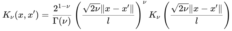
Where:

• ∥x−x′∥ is the Euclidean distance between the two points
• ν is the smoothness controlling parameter
• l is the length scale parameter (similar to the one in the RBF kernel)
• Γ(ν) is the Gamma function
• K ν  is the modified Bessel function of the second kind

The gamma function and the Bessel function are a bit wonkish, and we will not get into them, however for our purposes we are having ν as ³/2 which makes our kernel, almost, halfway between an exponential kernel and the Radial Basis Function Kernel. When we do that, our formula for the Matérn kernel simplifies to:

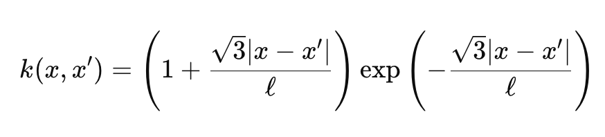
Where

• Representations are similar to the first formula shared above.

Special cases:

• For ν=¹/2, the Matérn kernel becomes the Exponential Kernel.
• For ν→∞, it becomes the RBF kernel.

The smoothness of this kernel is very sensitive to the ν parameter, and typically it gets assigned either ¹/2  or ³/2  or ⁵/2 . Each of these parameter values implies a different degree of smoothness, with a larger value leading to more smoothness.

When v is ¹/2  the kernel is equivalent to the exponential kernel as mentioned and this makes it suitable for modelling data sets where sharp changes or discontinuities are common place. From a trader’s perspective, this usually points to very volatile securities or forex pairs. This kernel setting assumes a jagged process and therefore tends to produce results that are less smooth and arguably more responsive to immediate changes. When v is ³/ 2  which is the setting we are adopting for this article when testing the wizard assembled Expert Advisor, its smoothness is often rated intermediate. It is a compromise in that it can handle both mildly volatile data and mildly trending data sets. This kind of setting, one could argue, makes the kernel suitable for determining turning points in a time series or swing points in the market. The ⁵/2  setting and anything higher makes the kernel a better fit for trending environments, especially when the rate is in question.

So, noisy data or data sets that have jumps or discontinuities are better served by the smaller ν values, while data sets that are more gradual and have smooth changes would work well with higher v values. As a side note, differentiability or the number of times the kernel function can be differentiated, increases with the v parameter. This in turn correlates with compute resources with higher ν parameter values, using up more compute. We implement the Matérn kernel in MQL5 as follows:

//+------------------------------------------------------------------+
// Matern Kernel Function
//+------------------------------------------------------------------+
matrix CSignalGauss::Matern_Kernel(vector &Rows,vector &Cols)
{  matrix _matern;
   _matern.Init(Rows.Size(), Cols.Size());
   for(int i = 0; i < int(Rows.Size()); i++)
   {  for(int ii = 0; ii < int(Cols.Size()); ii++)
      {  _matern[i][ii] = (1.0 + (sqrt(3.0) * fabs(Rows[i] - Cols[ii]) / m_next)) * exp(-1.0 * sqrt(3.0) * fabs(Rows[i] - Cols[ii]) / m_next);
      }
   }
   return(_matern);
}

When compared to linear kernels, therefore, Matérn kernels are more flexible and better suited for capturing complex, non-linear data relationships. When modelling a lot of real-world phenomena & data it clearly has an advantage over linear kernels because as we have seen above, slight tuning/ adjustment of the v parameter makes it capable of not just handling trending data sets but also volatile and discontinuous data as well.

The Signal Class

We create a custom signal class that brings together the two kernels as two implementation options in the signal class. Our get output function is also re-coded to cater for the choice of kernel selection from the Expert Advisor’s input. The new function is as follows:

//+------------------------------------------------------------------+
//|                                                                  |
//+------------------------------------------------------------------+
void CSignalGauss::GetOutput(double BasisMean, vector &Output)
{  

   ...

   matrix _k_s;
   matrix _k_ss;
   _k_s.Init(_next_time.Size(), _past_time.Size());
   _k_ss.Init(_next_time.Size(), _next_time.Size());
   if(m_kernel == KERNEL_LINEAR)
   {  _k_s = Linear_Kernel(_next_time, _past_time);
      _k_ss = Linear_Kernel(_next_time, _next_time);
   }
   else if(m_kernel == KERNEL_MATERN)
   {  _k_s = Matern_Kernel(_next_time, _past_time);
      _k_ss = Matern_Kernel(_next_time, _next_time);
   }

   ...

}

The steps involved in interpolating the next price changes, once the appropriate kernel has been selected, are identical to what we covered in this earlier article. The long condition as well as short condition processing are also not very different, and their code is shared here for completeness:

//+------------------------------------------------------------------+
//| "Voting" that price will grow.                                   |
//+------------------------------------------------------------------+
int CSignalGauss::LongCondition(void)
{  int result = 0;
   vector _o;
   GetOutput(0.0, _o);
   if(_o[_o.Size()-1] > _o[0])
   {  result = int(round(100.0 * ((_o[_o.Size()-1] - _o[0])/(_o.Max() - _o.Min()))));
   }
//printf(__FUNCSIG__ + " output is: %.5f, change is: %.5f, and result is: %i", _mlp_output, m_symbol.Bid()-_mlp_output, result);return(0);
   return(result);
}
//+------------------------------------------------------------------+
//| "Voting" that price will fall.                                   |
//+------------------------------------------------------------------+
int CSignalGauss::ShortCondition(void)
{  int result = 0;
   vector _o;
   GetOutput(0.0, _o);
   if(_o[_o.Size()-1] < _o[0])
   {  result = int(round(100.0 * ((_o[0] - _o[_o.Size()-1])/(_o.Max() - _o.Min()))));
   }
//printf(__FUNCSIG__ + " output is: %.5f, change is: %.5f, and result is: %i", _mlp_output, m_symbol.Bid()-_mlp_output, result);return(0);
   return(result);
}

The conditions as in the linked article are based on whether the forecast price change is going to be positive or negative. These changes are then normalized to be in the 0 to 100 integer range, as is expected of all custom signal class instances. The assembly of this signal file into an Expert Advisor via the MQL5 wizard is covered in separate articles here and here for readers that are new.

Strategy Tester Reports

We perform some optimizations, on the pair GBPJPY, on the daily time frame for the year 2023 with the linear kernel and with the Matérn kernel. The results from each, that simply demonstrate the usability of the Expert Advisor but do not in any way point to future performance, are indicated below:

And the results for the Matérn kernel are:

An alternative implementation of both kernels can also be with a custom money management class. This also like the signal can be assembled in the MQL5 wizard with the difference being that only one custom instance of money management is selected. To use the Gaussian Process regression as we did with the signal class, we would ideally have a common anchor class that is referenced by both the custom signal class and the custom money management class. This would minimize duplicity in coding of the same functions that perform very similar tasks in the two custom classes.

However, in the money management class, we have some slight changes in the type of data that is fed to the Gaussian Process kernels. Whereas we had close price changes as the input data set for the custom signal class, for this money management class we have changes in the ATR indicator as inputs to our kernel. The output for our kernel is trained to be the next change in the ATR. This custom class is also an adaptation from the common money-size optimized class that, for those who may be unfamiliar, is built to reduce position size if an Expert Advisor sustains a run of losses. The proportion of reduction in lot sizes is proportional to the string of losses sustained. We adopt this class and make some changes governing when the reduction in lots takes place.

With our modifications, we only reduce the lots if the Expert Advisor sustains losses and there is a projection for rising ATR across the forecast values. The number of these forecast values is set by the parameter ‘m_next’ as discussed in the already linked article, that introduced Gaussian Process Regression in these series. These changes together with most of the original code for optimizing the position size is shared below:

//+------------------------------------------------------------------+
//| Optimizing lot size for open.                                    |
//+------------------------------------------------------------------+
double CMoneyGAUSS::Optimize(int Type, double lots)
{  double lot = lots;
//--- calculate number of losses orders without a break
   if(m_decrease_factor > 0)
   {  //--- select history for access
      HistorySelect(0, TimeCurrent());
      //---
      int       orders = HistoryDealsTotal(); // total history deals
      int       losses = 0;                  // number of consequent losing orders
      //--
      int      size = 0;
      matrix series;
      series.Init(fmin(m_series_size, orders), 2);
      series.Fill(0.0);
      //--
      CDealInfo deal;
      //---
      for(int i = orders - 1; i >= 0; i--)
      {  deal.Ticket(HistoryDealGetTicket(i));
         if(deal.Ticket() == 0)
         {  Print("CMoneySizeOptimized::Optimize: HistoryDealGetTicket failed, no trade history");
            break;
         }
         //--- check symbol
         if(deal.Symbol() != m_symbol.Name())
            continue;
         //--- check profit
         double profit = deal.Profit();
         //--
         series[size][0] = profit;
         size++;
         //--
         if(size >= m_series_size)
            break;
         if(profit < 0.0)
            losses++;
      }
      //--
      double _cond = 0.0;
      //--
      vector _o;
      GetOutput(0.0, _o);
      //---
      //decrease lots on rising ATR
      if(_o[_o.Size()-1] > _o[0])
         lot = NormalizeDouble(lot - lot * losses / m_decrease_factor, 2);
   }
//--- normalize and check limits
   double stepvol = m_symbol.LotsStep();
   lot = stepvol * NormalizeDouble(lot / stepvol, 0);
//---
   double minvol = m_symbol.LotsMin();
   if(lot < minvol)
      lot = minvol;
//---
   double maxvol = m_symbol.LotsMax();
   if(lot > maxvol)
      lot = maxvol;
//---
   return(lot);
}

A similar approach can also be taken when creating a custom trailing class that utilizes Gaussian Process kernels, as we have demonstrated above. There is a variety of indicators to choose from, besides the easy price access that is afforded by the vector and matrix data types.

Conclusion

To conclude, we have continued our delve into Gaussian Process Regression by considering another set of kernels that can be used with this form of regression when making forecasts with financial time series. The linear kernel and the Matérn kernel are almost opposites not only in the types of data sets they are suited for but also in their flexibility. While the linear kernel can only handle a given type of data set, it is often practical to start modelling with it, especially in cases where the data set samples could be small in size at the onset of a study. With time once the data set sample increases and the data becomes more complex, or even noisy then a more robust kernel like the Matérn kernel can be utilized to not only handle the noisy data or gaps or discontinuations, but also data sets that could be very smooth. This is because the adjustability of its key input parameter v allows it to assume different roles depending on the challenges presented by the data set, and that’s why it is arguably better suited for most data environments.