MQL5 Wizard Techniques you should know (Part 36): Q-Learning with Markov Chains

Introduction

Custom signal classes for wizard assembled Expert Advisors can take on various roles, that are worth exploring, and we continue this quest by examining how the Q-Learning algorithm when paired with Markov Chains can help refine the learning process of a multi-layer-perceptron network. Q-Learning is one of the several (approximately 12) algorithms of reinforcement-learning, so essentially this is also a look at how this subject can be implemented as a custom signal and tested within a wizard assembled Expert Advisor.

So, the structure for this article will flow from what is reinforcement-learning, dwell on the Q-Learning algorithm and its cycle stages, look at how Markov chains can be integrated into Q-Learning, and then conclude as always with strategy tester reports. Reinforcement learning can be utilized as an independent signal generator because its cycles (‘episodes’) are in essence a form of learning that quantifies results as ‘rewards’ for each of the ‘environments’ the ‘actor’ is involved in. These terms in quotes are introduced below. We, however, are not using reinforcement learning as a raw signal, but rather are relying on its abilities to further the learning process by having it supplement a multi-layer-perceptron.

Given reinforcement-learning’s position as the third standard in machine learning training besides supervised learning and unsupervised learning I thought we could have it involved more in the loss function of an MLP since it in a sense acts as a go between supervision and no-supervision by using ‘critic-rewards’ and ‘environment-states’ respectively. Both quoted terms are introduced in the next section; however, this means most of the forecasting is still up to the MLP and reinforcement learning is playing more of a subordinate role. In addition, the use of Markov Chains is also supplementary to the reinforcement learning as the ‘actor’ selections from the ‘Q-Map’ are often sufficient in implementing the Q-Learning algorithm however we include it here to get a sense of the difference, if any, in test results it provides.

Overview of Reinforcement Learning

Reinforcement learning, which we have introduced above as the third leg to the stool of machine learning training, is a way of balancing both Exploration and Exploitation during the training process. This is made possible thanks to its cyclical approach at appraising each training round, where training rounds are referred to as episodes. This cycle can be represented in the diagram below:

source

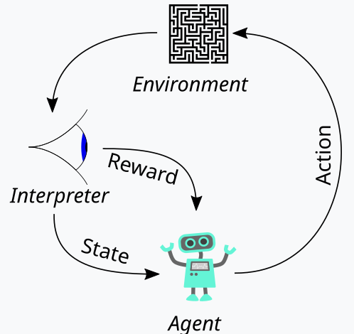
So, with this, we have a sequence of steps in the reinforcement learning process. At the onset, is an ‘Agent’, that acts on behalf of a primary party who in our case is an MLP, to select the ideal course of action when faced with an updated Q-Learning map or kernel or matrix.  This map is a record of all the possible environment states plus a probability distribution over what possible actions to take for each of the available states.

The best way to illustrate this could be if we walk through the implementation of the environment that we have chosen for this article. As traders, we often look to define markets not just by their short-term action, but also by their trendy or long-term traits. So, we if we focus on 3 basic metrics namely bullishness, bearishness, and flatness, then each of these three can have indicators on a shorter time frame and a longer time frame. So, in essence our ‘environment’ is a 9-index space (3 x 3 for short-term by long-term) where an index like 0 marks bearishness in the short-term and long-term, the index 4 marks a sideways market in both the short-term and long-term, while the index 8 marks bullishness on both time horizons etc.

The environments are selected with the help of a like named function, whose source is given below:

//+------------------------------------------------------------------+
// Indexing new Environment data to conform with states
//+------------------------------------------------------------------+
void Cql::Environment(vector &E_Row, vector &E_Col, vector &E)
{  if(E_Row.Size() == E_Col.Size() && E_Col.Size() > 0)
   {  E.Init(E_Row.Size());
      E.Fill(0.0);
      for(int i = 0; i < int(E_Row.Size()); i++)
      {  if(E_Row[i] > 0.0 && E_Col[i] > 0.0)
         {  E[i] = 0.0;
         }
         else if(E_Row[i] > 0.0 && E_Col[i] == 0.0)
         {  E[i] = 1.0;
         }
         else if(E_Row[i] > 0.0 && E_Col[i] < 0.0)
         {  E[i] = 2.0;
         }
         else if(E_Row[i] == 0.0 && E_Col[i] > 0.0)
         {  E[i] = 3.0;
         }
         else if(E_Row[i] == 0.0 && E_Col[i] == 0.0)
         {  E[i] = 4.0;
         }
         else if(E_Row[i] == 0.0 && E_Col[i] < 0.0)
         {  E[i] = 5.0;
         }
         else if(E_Row[i] < 0.0 && E_Col[i] > 0.0)
         {  E[i] = 6.0;
         }
         else if(E_Row[i] < 0.0 && E_Col[i] == 0.0)
         {  E[i] = 7.0;
         }
         else if(E_Row[i] < 0.0 && E_Col[i] < 0.0)
         {  E[i] = 8.0;
         }
      }
   }
}

This code strictly applies to our 9-index environment and cannot be used in environment matrices of different size. In defining this environment matrix, we use an extra input parameter referred to as ‘scale’. This scale helps proportion or ratio our long-time frame horizon to our short-term frame window. The default value for this is 5 which means on one axis of the environment matrix we mark off the state as either bullish, flat or bearish based on the changes in price over a period that is 5 times longer than another period whose values are ‘plotted’ on the other axis. I say ‘plotted’ because these two axes simply provide coordinate points for the current state. The indexing from 0 to 8 is simply a flattening of this matrix into an array, but as you can see from the attached source code, the continuous reference to ‘row’ and ‘col’ simply points to the possible x and y coordinate readings from the environment matrix that define the current state.

The Q-Learning map reproduces this array of environment states by adding weighting for what possible actions to take in any of these environment states. Because in our case we are looking at 3 possible actions that can be taken in each state, namely buying, selling or doing nothing, each state in the Q-Learning map has a 3-sized array that keeps score of which action is most suitable. The higher the score value, the more suitable it is. The other major entity in our cycle diagram above is the observer, whom we will refer to as the ‘critic’. It is the critic that is firstly charged with determining the ‘rewards’ for the actor’s actions. And what are rewards? Well, this will depend on what the reinforcement learning is used for but for our purposes, based on the possible 3 actions of the actor, we are using the raw tick value profits from price change as the reward.

So, if this price change is negative and our last action was to sell, then the magnitude of this change acts as a reward. The same would be applied if the change is positive following a previous buy action. If, however the last action was a buy, and we have a negative price change then the size of this negative value acts as a penalty in the same way that price changes following a sell are always multiplied by negative one meaning any resulting negative product would act as a penalty to our actions at that particular state (which is our environment or the indexing of short-term and long-term price action of the market).  

This reward value needs to be normalized, though, and that’s why we use the critic-reward function that keeps it in the range 0.0 to 1.0. All negative values are from 0.0 to 0.5 while positive values are normalized to 0.5 to 1.0. The source code that does this is given below:

//+------------------------------------------------------------------+
// Normalize reward via off-policy
//+------------------------------------------------------------------+
double Cql::CriticReward(double MaxProfit, double MaxLoss, double Float)
{  double _reward = 0.0;
   if(MaxProfit >= Float && Float >= MaxLoss && MaxLoss < MaxProfit)
   {  _reward = (Float - MaxLoss) / (MaxProfit - MaxLoss);
   }
   return(_reward);
}

The updating of the reward value would always occur mid the training process and not once at the beginning. This implies we constantly need to be passing on parameters that update the values of reward-max, reward-min and reward-float to the back-propagation function so that they can be incorporated into the process. To accomplish this, we start by modifying the learning struct, that is used to store learning variables that are callable on each back-propagation run. The use of a struct actually makes our code easily modifiable, since we only have to add the extra new variables we need to the existing list of variables within the struct. This is clearly less error-prone and contrasts sharply with having to modify the list of input parameters into a function that requires the variables in this struct. It would certainly be unwieldy then. The modified learning struct now looks as follows:

//+------------------------------------------------------------------+
//| Learning Struct                                                  |
//+------------------------------------------------------------------+
struct Slearning
{  Elearning         type;
   int               epochs;
   double            rate;
   double            initial_rate;
   double            prior_rate;
   double            min_rate;
   double            decay_rate_a;
   double            decay_rate_b;
   int               decay_epoch_steps;
   double            polynomial_power;
   double            ql_reward_max;
   double            ql_reward_min;
   double            ql_reward_float;
   vector            ql_e;

                     Slearning()
   {  type = LEARNING_FIXED;
      rate = 0.005;
      prior_rate = 0.1;
      epochs = 50;
      initial_rate = 0.1;
      min_rate = __EPSILON;
      decay_rate_a = 0.25;
      decay_rate_b = 0.75;
      decay_epoch_steps = 10;
      polynomial_power = 1.0;
      ql_reward_max = 0.0;
      ql_reward_min = 0.0;
      ql_reward_float = 0.0;
      ql_e.Init(1);
      ql_e.Fill(0.0);
   };
                    ~Slearning() {};
};

In addition, we have to make some changes in the back-propagation function at the time we call the loss function. This is because we have now introduced a new or subordinate enumeration for loss functions, whose listing is as follows:

//+------------------------------------------------------------------+
//| Custom Loss-Function Enumerator                                  |
//+------------------------------------------------------------------+
enum Eloss
{  LOSS_TYPICAL = -1,
   LOSS_SVR = 1,
   LOSS_QL = 2
};

One of the enumerations is ‘LOSS_SVR’ which deals with measuring the loss using support vector regression, an approach we tackled in the last article. The other two are ‘LOSS_TYPICAL’ loss which when selected defaults to the list of inbuilt loss functions in MQL5, and the other being ‘LOSS_QL’ where QL stands for Q-Learning and when this is selected then reinforcement learning with Q-learning informs the learning process by providing a target (or label) vector to which the MLP forecasts can be compared. If clauses within the back-propagation function do check for this as follows:

//+------------------------------------------------------------------+
//| BACKWARD PROPAGATION OF THE MULTI-LAYER-PERCEPTRON.              |
//+------------------------------------------------------------------+
//|                                                                  |
//| -Extra Validation check of MLP architecture settings is performed|
//|  at run-time.                                                    |
//|  Chcecking of 'validation' parameter should ideally be performed |
//|  at class instance initialisation.                               |
//|                                                                  |
//| -Run-time Validation of learning rate, decay rates and epoch     |
//|  index is performed as these are optimisable inputs.             |
//+------------------------------------------------------------------+
void Cmlp::Backward(Slearning &Learning, int EpochIndex = 1)
{  

   ...

   if(THIS.loss_custom == LOSS_SVR)
   {  _last_loss = SVR_Loss();
   }
   else if(THIS.loss_custom == LOSS_QL)
   {  double _reward = QL.CriticReward(Learning.ql_reward_max, Learning.ql_reward_min, Learning.ql_reward_float);
      if(QL.act == 0)
      {  _reward *= -1.0;
      }
      else if(QL.act == 1)
      {  _reward = -1.0 * fabs(_reward);
      }
      QL.CriticState(_reward, Learning.ql_e);
      _last_loss = output.LossGradient(QL.Q_Loss(), THIS.loss_typical);
   }
   

...

}

The addition of this custom loss function does not necessarily negate the need for the old loss functions that were used based on the inbuilt enumerations within MQL5. We have simply renamed it from loss to ‘typical_loss’ and if the input ‘custom_loss’ is ‘LOSS_TYPICAL’ then this value would have to be provided.

After the reward value is normalized, it is used to update the Q-Learning map in the critic-state function. The updating of the Q values is governed by the following formula:

Where:

• Q(s,a): The Q-value for taking action a in state s. This represents the expected future reward for that state-action pair.
• α: The learning rate, a value between 0 and 1, which controls how much new information overrides the old information. A smaller α means the agent learns more slowly, while a larger α makes it more responsive to recent experiences.
• r: The most recent reward received after taking action a in state s.
• γ: The discount factor, a value between 0 and 1, that discounts future rewards. A higher γ makes the agent values long-term rewards more, while a lower γ makes it focus more on immediate rewards.
• max a′ ​Q(s′,a′): The maximum Q-value for the next state s′ over all possible actions a′ This represents the agent's estimate of the best possible future reward starting from the next state s′

And the actual updating of the Q-Learning map can be implemented in MQL5 as follows:

//+------------------------------------------------------------------+
// Update Q-value using off-policy (Q-learning formula)
//+------------------------------------------------------------------+
void Cql::CriticState(double Reward, vector &E)
{  int _e_row_new = 0, _e_col_new = 0;
   SetMarkov(int(E[E.Size() - 1]), _e_row_new, _e_col_new);
   e_row[1] = e_row[0];
   e_col[1] = e_col[0];
   e_row[0] = _e_row_new;
   e_col[0] = _e_col_new;
   int _new_best_q = Action();
   double _weighting = Q[e_row[0]][e_col[0]][_new_best_q];
   if(THIS.use_markov)
   {  LetMarkov(e_row[1], e_col[1], E);
      int _old_index = GetMarkov(e_row[1], e_col[1]);
      int _new_index = GetMarkov(e_row[0], e_col[0]);
      _weighting *= markov[_old_index][_new_index];
   }
   Q[e_row[1]][e_col[1]][act] += THIS.alpha * (Reward + (THIS.gamma * _weighting) - Q[e_row[1]][e_col[1]][act]);
}

In updating the map, the off-policy rule of updating where the best action of the next state is used to update the old action, is applied. This contrasts with on-policy action, where the current action is used in the next state to do the same update. This is because for any state, that is defined by a row coordinate, and a column coordinate within the environment matrix, there is a standard array of possible actions the agent can perform. And with off-policy updates which is what Q-Learning uses, the best weighted action is chosen however with algorithms that use on-policy updates, the current action is maintained in performing the update. The selecting of the best action is performed via the ‘Action’ function, whose code is given below:

//+------------------------------------------------------------------+
// Choose an action using epsilon-greedy
//+------------------------------------------------------------------+
int Cql::Action()
{  int _best_act = 0;
   if (double((rand() % SHORT_MAX) / SHORT_MAX) < THIS.epsilon)
   {  // Explore: Choose random action
      _best_act = (rand() % THIS.actions);
   }
   else
   {  // Exploit: Choose best action
      double _best_value = Q[e_row[0]][e_col[0]][0];
      for (int i = 1; i < THIS.actions; i++)
      {  if (Q[e_row[0]][e_col[0]][i] > _best_value)
         {  _best_value = Q[e_row[0]][e_col[0]][i];
            _best_act = i;
         }
      }
   }
   //update last action
   act = _best_act;
   return(_best_act);
}

Reinforcement learning is a bit like supervised learning in that there is a reward metric that is used to adjust and fine tune the weighting of actions at each environment state. On the other hand, as well, it is as if unsupervised learning given the use of an environment matrix whose coordinate values, (the two values for the row index and column index) serve as inputs to the MLP that uses it. The MLP therefore serves as a classifier that tries to determine the correct probability distribution for the three applicable actions when presented with environment state coordinates as inputs. The training then happens as in any classifier MLP, but this time we aim to minimize the difference between the projected probability distribution of the MLP and the probability distribution in the Q-Learning kernel at the Q-Learning map coordinates provided as input to the MLP.

The role of Markov Transitions

Markov chains are probability stochastic models that use transition matrices to map probabilities of moving from one state to another when fed with a time-series sequence of these states. These probability models are inherently memoryless, since the probability of transitioning to the next state is solely based on the current state and not on the history of states before it. These transitions can be used to attach importance to the various states that are defined within the environment matrix.

Now the environment matrix, from our use case in the custom signal only considers the three market states of bullishness, bearishness and flatness on a short horizon and long-time frame making it a 3 x 3 matrix which thus implies nine possible states. Because we have nine possible states, this means our Markov transition matrix will be a 9 x 9 matrix in order to map the transitions from one environment state to another. This therefore necessitates being able to convert the pair of indices in the environment matrix into a single index that is usable in the Markov transition matrix. We actually end up needing two functions, one to convert the pair of environment row and column indices into a single index for the Markov matrix and another to reconstruct the row and column indices of the environment matrix when presented with a Markov transition matrix index. These two functions are named Get Markov and Set Markov respectively and their source is given below:

//+------------------------------------------------------------------+
// Getting markov index from environment row & col
//+------------------------------------------------------------------+
int Cql::GetMarkov(int Row, int Col)
{  return(Row + (THIS.environments * Col));
}

And:

//+------------------------------------------------------------------+
// Getting environment row & col from markov index
//+------------------------------------------------------------------+
void Cql::SetMarkov(int Index, int &Row, int &Col)
{  Col = int(floor(Index / THIS.environments));
   Row = int(fmod(Index, THIS.environments));
}

We need to get the Markov equivalent index of the two environment state coordinates at the start of performing the Markov calculations, since we would be transitioning from this state. Once we get that index, we then retrieve the probabilities of transitioning to other states along this column in the transition matrix, since each of them serves as a weight. As expected, they all add up to one and since the actor has already selected the next state from the Q-Map we use its probability as the numerator to a denominator of one meaning only its probability is used as a weight to increment the new value in the Q-Map during the learning process. Source code implementing this is already shared above in the critic state function.

This learning process essentially discounts the learning increment in proportion to its probability in the Markov transition matrix.

In addition, we perform the transition matrix calculations whenever a new-bar is registered and the time series of prices receives an update. The code for performing these calculations is given below:

//+------------------------------------------------------------------+
// Function to update markov matrix
//+------------------------------------------------------------------+
void Cql::LetMarkov(int OldRow, int OldCol, vector &E)  //
{  matrix _transitions;  // Count the transitions
   _transitions.Init(markov.Rows(), markov.Cols());
   _transitions.Fill(0.0);
   vector _states;  // Count the occurrences of each state
   _states.Init(markov.Rows());
   _states.Fill(0.0);
// Count transitions from state i to state ii
   for (int i = 0; i < int(E.Size()) - 1; i++)
   {  int _old_state = int(E[i]);
      int _new_state = int(E[i + 1]);
      _transitions[_old_state][_new_state]++;
      _states[_old_state]++;
   }
// Reset prior values to zero.
   markov.Fill(0.0);
// Compute probabilities by normalizing transition counts
   for (int i = 0; i < int(markov.Rows()); i++)
   {  for (int ii = 0; ii < int(markov.Cols()); ii++)
      {  if (_states[i] > 0)
         {  markov[i][ii] = double(_transitions[i][ii] / _states[i]);
         }
         else
         {  markov[i][ii] = 0.0;  // No transitions from this state
         }
      }
   }
}

Being a memoryless transition matrix, our code above always begins with a newly declared matrix and the class variable that holds the probabilities also gets filled with zero values to cancel out any prior history. The approach in computing the transitions is straightforward, since we get a count of each state's sequence in the first for loop, and we follow this with another for loop that divides the cumulative counts we got for each transition by the total number of states from which transitions are made.

Implementing the custom signal class

As mentioned already we are using an MLP that is a classifier to handle the main forecasting with reinforcement-learning only serving in a subordinate role as a loss function. Reinforcement learning can also be optimized or trained to output usable trade signals by maximizing the critic rewards however that is not what we are doing here instead its role is secondary to the multi-layer perceptron since like in supervised learning as well as in unsupervised, it is used to quantify the objective function.

As we have in past articles where we have used MLPs, we are using price changes as the origin for our data input. Recall, the environment matrix used for this article is a 3 x 3 matrix that serves as a grid of possible states of the market when weighed on the short-timeframe and the long-timeframe. Each of the axes for the short-timeframe and the long-timeframe have metrics or readings from bullishness to flat to bearishness, which constitute the 3 x 3 grid. And similar to this matrix is the Q-Learning matrix or map that also has this 3 x 3 grid with the addition of an array of possible actions, open to the actor, that keep score of the suitability of each action for each state. It is this suitability array that serves as the label or training target to our MLP.

The inputs to the MLP though will not be raw price changes as had been the case in our recent articles with MLP, but rather they will be the environment state coordinates for the most recent or current price change over the short-timeframe and long-timeframe. The use of ‘timeframe’ here is purely to illustrate the different time scales or horizons over which price changes are measured. We do not have two separate timeframes as inputs to the signal class that guide the measuring of these changes, but rather we have a single input integer parameter that is labelled ‘m_scale’ that is a multiple of how much larger the ‘long-timeframe’ is to the short. Since the short-timeframe uses changes across a single price bar, the ‘long-timeframe’ gets is change readings over a period equivalent to this scale input parameter. This processing is performed in the get output function as follows:

//+------------------------------------------------------------------+
//|                                                                  |
//+------------------------------------------------------------------+
void CSignalQLM::GetOutput(int &Output)
{  m_learning.rate = m_learning_rate;
   for(int i = m_epochs; i >= 1; i--)
   {  MLP.LearningType(m_learning, i);
      for(int ii = m_train_set; ii >= 0; ii--)
      {  vector _in, _in_row, _in_row_old, _in_col, _in_col_old;
         if
         (
            _in_row.Init(m_scale) &&
            _in_row.CopyRates(m_symbol.Name(), m_period, 8, ii + 1, m_scale) &&
            _in_row.Size() == m_scale
            &&
            _in_row_old.Init(m_scale) &&
            _in_row_old.CopyRates(m_symbol.Name(), m_period, 8, ii + 1 + 1, m_scale) &&
            _in_row_old.Size() == m_scale
            &&
            _in_col.Init(m_scale) &&
            _in_col.CopyRates(m_symbol.Name(), m_period, 8, ii + 1, m_scale) &&
            _in_col.Size() == m_scale
            &&
            _in_col_old.Init(m_scale) &&
            _in_col_old.CopyRates(m_symbol.Name(), m_period, 8, m_scale + ii + 1, m_scale) &&
            _in_col_old.Size() == m_scale
         )
         {  _in_row -= _in_row_old;
            _in_col -= _in_col_old;
            vector _in_e;
            _in_e.Init(m_scale);
            MLP.QL.Environment(_in_row, _in_col, _in_e);
            int _row = 0, _col = 0;
            MLP.QL.SetMarkov(int(_in_e[m_scale - 1]), _row, _col);
            _in.Init(__MLP_INPUTS);
            _in[0] = _row;
            _in[1] = _col;
            MLP.Set(_in);
            MLP.Forward();
            if(ii > 0)
            {  vector _target, _target_data;
               if
               (
                  _target_data.Init(2) &&
                  _target_data.CopyRates(m_symbol.Name(), m_period, 8, ii, 2) &&
                  _target_data.Size() == 2
               )
               {  _target.Init(__MLP_OUTPUTS);
                  _target.Fill(0.0);
                  double _type = _target_data[0] - _in_row[1];
                  int _index = (_type < 0.0 ? 0 : (_type > 0.0 ? 2 : 1));
                  _target[_index] = 1.0;
                  MLP.Get(_target);
                  m_learning.ql_e = _in_e;
                  m_learning.ql_reward_float = _in_row[m_scale - 1];
                  m_learning.ql_reward_max = _in_row.Max();
                  m_learning.ql_reward_min = _in_row.Min();
                  if(i == m_epochs && ii == m_train_set)
                  {  MLP.QL.Action();
                  }
                  MLP.Backward(m_learning, i);
               }
            }
            Output = (MLP.output.Max()==MLP.output[0]?0:(MLP.output.Max()==MLP.output[1]?1:2));
         }
      }
   }
}

So, as we can see from our source code above, we need 4 vectors to get the coordinate readings for our MLP inputs. Once these are determined, with the help of the Environment function that converts the two price changes into a single Markov index and the set Markov function that provides these two coordinates from the MARKOV index, we fill them into the ‘in’ vector that is our input. The MLP classifier has a very basic architecture of 2-8-3 which represents 2 inputs, 8-sized hidden layer and 3 outputs that correspond to the three possible actions open to the actor. The output of the MLP is essentially a probability map that gives values for either going short (under index 0), doing nothing (under index 1) and going long (under index 2).

The reinforcement-learning training process measures how far these outputs are from the similar vectors attached to each environment state.  

Strategy Tester Results

So, as always, we perform optimizations and test runs with real-tick data purely for purposes of demonstrating how an Expert Advisor that is assembled via the MQL5 wizard with this signal class could be able to perform its basic functions. Guides on using the attached code with the MQL5 wizard can be found here and here. A lot of diligence work in making the assembled Expert Advisor or trade system live-account ready is not handled in these articles and is left to the reader. We perform runs on the pair GBPJPY for the year 2023 on the daily time frame. We have introduced Markov Chains as an alternative to weighting the Q-Learning map values, and therefore we run two tests, one without the Markov chain weighting and one with the weighting. And here are the results:

  And then the results without Markov weighting are: 

These test results are not achieved with the best optimization settings nor are walk-forward tests performed with these settings; therefore they are not an endorsement for the supplemental use of Markov chains with Q-Learning per se, although sound arguments and a more comprehensive testing regime can make the case for its use.

Conclusion

For this article, we have highlighted what else could be possible with the MQL5 wizard by introducing reinforcement learning, an alternative in machine-learning training besides the established methods of supervised learning and unsupervised learning. We have sought to use this in the training of a classifier MLP by having it inform and guide the training process rather than by having it as the raw signal generator, which is also possible. In doing so, while focusing on the Q-Learning algorithm, we exploited Markov-Chains, a transition probability matrix, that can act as a weight to the reinforcement-learning training process, and we have presented test runs of a trading Expert Advisor in 2 scenarios; when trained without the Markov chains, and when trained with them.

This has been, I think, a bit more complex compared to my earlier articles seeing as we are referencing 2 classes to our custom signal and a lot of sensitive input parameters have been used with their default values without any major tuning, plenty of new terms needed introduction for those unfamiliar with the subject. However, it is the beginning of our tackling of this broad and deep subject, reinforcement-learning, and so I hope in future articles when we re-visit this subject it will not be as daunting.