Gain An Edge Over Any Market (Part II): Forecasting Technical Indicators

Introduction

Investors seeking to apply machine learning in electronic trading environments face numerous challenges, and the reality is that many do not achieve their desired outcomes. This article aims to highlight some reasons why, in my opinion, an aspiring algorithmic trader may fail to achieve satisfactory returns relative to the complexity of their strategies. I will demonstrate why forecasting the price of a financial security often struggles to exceed 50% accuracy and how focusing on predicting technical indicator values, instead, can improve accuracy to around 70%. This guide will provide step-by-step instructions on best practices for time series analysis.

By the end of this article, you will have a solid understanding of how to enhance the accuracy of your machine learning models and discover leading indicators of market changes more effectively than other participants using Python and MQL5.

Forecasting Indicator Values

We will fetch historical data from our MetaTrader 5 terminal and analyze it using standard Python libraries. This analysis will show that forecasting changes in indicator values is more effective than predicting security price changes. This is true because we can only partially observe the factors influencing a security's price. In reality, we cannot model every single variable affecting the price of a symbol due to their sheer number and complexity. However, we can fully observe all the factors affecting the value of a technical indicator.

First, I'll demonstrate the principle and then explain why this approach works better at the end of our discussion. By seeing the principle in action first, the theoretical explanation will be easier to understand. Let's start by selecting the symbol list icon in the menu just above the chart.

Our goals here are focused on fetching data:

• Open your MetaTrader 5 terminal.
• Select the symbol list icon in the menu above the chart.
• Choose the desired symbol and time frame for your analysis.
• Export the historical data to a comma separated value (csv) file.

Fig 1: Getting historical data.

Search for the symbol you'd like to model.

Fig 2: Searching for your desired symbol.

Afterward, select the 'bars' tile in the menu, and make sure to request as much data as possible.

Fig 3: Requesting historical data.

Select export bars at the bottom menu so we can begin analyzing our data in Python.

,

Fig 4: Exporting our historical data.

As usual, we begin by first importing libraries we will need.

#Load libraries
import pandas as pd
import numpy as np
import matplotlib.pyplot as plt

Next, we read in our historical market data. Note that the MetaTrader 5 terminal exports csv files that are tab delimited, therefore we pass the tab notation to the separator parameter of our call to pandas read csv.

#Read the data
csv = pd.read_csv("/content/Volatility 75 Index_M1_20190101_20240131.csv",sep="\t")
csv

After reading in our historical data, it will look like this. We need to reformat the column titles a little and also add a technical indicator.

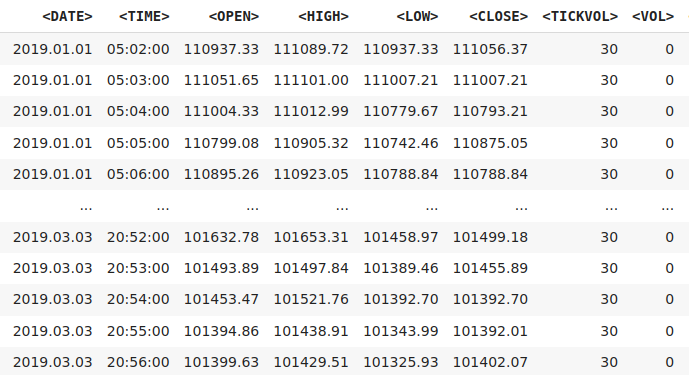
Fig 5: Our historical data from our MetaTrader 5 terminal.

We will now rename the columns.

#Format the data
csv.rename(columns={"<DATE>":"date","<TIME>":"time","<TICKVOL>":"tickvol","<VOL>":"vol","<SPREAD>":"spread","<OPEN>":"open","<HIGH>":"high","<LOW>":"low","<CLOSE>":"close"},inplace=True)
csv.ta.sma(length= 60,append=True)
csv.dropna(inplace=True)
csv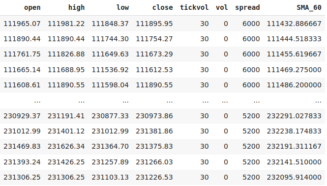

Fig 6: Formatting our data.

Now we can define our inputs.

#Define the inputs
predictors = ["open","high","low","close","SMA_60"]

Next, we will scale our data so that our model can train sufficiently.

#Scale the data
csv["open"] = csv["open"] /csv.loc[0,"open"]
csv["high"] = csv["high"] /csv.loc[0,"high"]
csv["low"] = csv["low"] /csv.loc[0,"low"]
csv["close"] = csv["close"] /csv.loc[0,"close"]
csv["SMA_60"] = csv["SMA_60"] /csv.loc[0,"SMA_60"]
    

We will approach this task as a classification problem. Our target will be categorical. A target value of 1 means the price of the security appreciated over 60 candles, and a target value of 0 means the price depreciated over the same horizon. Notice that we have two targets. One target is for monitoring the change in the close price, whilst the other is for monitoring the change in the moving average.

We will use the same encoding pattern on the changes in the moving average, a target value of 1 means the future moving average value in the next 60 candles will be greater, and conversely a target value of 0 means the moving average value will fall over the next 60 candles.

#Define the close
csv["Target Close"] = 0
csv["Target MA"] = 0

Define how far into the future you'd like to forecast.

#Define the forecast horizon
look_ahead = 60

Encode the target values.

#Set the targets
csv.loc[csv["close"] > csv["close"].shift(-look_ahead) ,"Target Close"] = 0
csv.loc[csv["close"] < csv["close"].shift(-look_ahead) ,"Target Close"] = 1
csv.loc[csv["SMA_60"] > csv["SMA_60"].shift(-look_ahead) ,"Target MA"] = 0
csv.loc[csv["SMA_60"] < csv["SMA_60"].shift(-look_ahead) ,"Target MA"] = 1
csv = csv[:-look_ahead]

We will fit the same group of models on the same dataset, remember that the only difference is that the first time our models will try to predict the change in close price whilst in the second test they will instead try to predict the change in a technical indicator, in our example the moving average.

After defining our targets, we can progress to import the models we need for our analysis.

#Get ready
from sklearn.discriminant_analysis import LinearDiscriminantAnalysis
from sklearn.linear_model import LogisticRegression
from xgboost import XGBClassifier
from sklearn.neural_network import MLPClassifier
from sklearn.metrics import accuracy_score
from sklearn.decomposition import PCA
from sklearn.model_selection import TimeSeriesSplit

We will prepare a time series split to evaluate where our validation error is lower. Additionally, we will transform our input data using the Principal Components Analysis (PCA) functions in sklearn. This step is necessary because our input columns may be correlated, which could hinder our model's learning process. By performing PCA, we transform our dataset into a form that ensures no correlation across the inputs, thereby improving our model's performance.

#Time series split
splits = 10
gap = look_ahead
models_close = ["Logistic Regression","LDA","XGB","Nerual Net Simple","Nerual Net Large"]
models_ma = ["Logistic Regression","LDA","XGB","Nerual Net Simple","Nerual Net Large"]
#Prepare the data
pca = PCA()
csv_reduced = pd.DataFrame(pca.fit_transform(csv.loc[:,predictors]))

Let us now observe our accuracy levels, using a neural network attempting to forecast changes in the close price directly.

#Fit the neural network predicting close price
model_close = MLPClassifier(solver='lbfgs',alpha=1e-5,hidden_layer_sizes=(5, 2), random_state=1)
model_close.fit(csv_reduced.loc[0:300000,:],csv.loc[0:300000,"Target Close"])
print("Close accuracy: ",accuracy_score(csv.loc[300070:,"Target Close"], model_close.predict(csv_reduced.loc[300070:,:])))

Close accuracy:  0.4990962620254304

Our accuracy when forecasting changes in the close price was 49.9%. This is not impressive considering the amount of complexity we've accepted, we could've gotten the same level of accuracy with a simpler model that is easier to maintain and understand, furthermore if we're only right 49% of the time then we will be in remain in an unprofitable position. Let us contrast this with our accuracy when forecasting changes in the moving average indicator.

#Fit the model predicting the moving average
model_ma = MLPClassifier(solver='lbfgs',alpha=1e-5,hidden_layer_sizes=(5, 2), random_state=1)
model_ma.fit(csv_reduced.loc[0:300000,:],csv.loc[0:300000,"Target MA"])
print("MA accuracy: ",accuracy_score(csv.loc[300070:,"Target MA"], model_ma.predict(csv_reduced.loc[300070:,:])))

MA accuracy:  0.6879839284668174

Our model's accuracy was 68.8% when forecasting the changes in the moving average, as opposed to 49.9% when forecasting the changes in price. This is an acceptable level of accuracy relative to the complexity of the modelling technique we are using.

We will now fit a variety of models and see which model can best predict changes in price and which model can best predict changes to the moving average.

#Error metrics
tscv = TimeSeriesSplit(n_splits=splits,gap=gap)
error_close_df = pd.DataFrame(index=np.arange(0,splits),columns=models_close)
error_ma_df = pd.DataFrame(index=np.arange(0,splits),columns=models_ma)

We will first assess the accuracy of each of our selected models trying to forecast the close price.

#Training each model to predict changes in the close price
for i,(train,test) in enumerate(tscv.split(csv)):
    model= MLPClassifier(solver='lbfgs',alpha=1e-5,hidden_layer_sizes=(20, 10), random_state=1)
    model.fit(csv_reduced.loc[train[0]:train[-1],:],csv.loc[train[0]:train[-1],"Target Close"])
    error_close_df.iloc[i,4] = accuracy_score(csv.loc[test[0]:test[-1],"Target Close"],model.predict(csv_reduced.loc[test[0]:test[-1],:]))

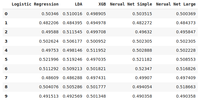
Fig 7: The accuracy results of different models trying to classify changes in price.

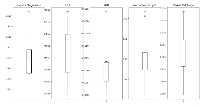
Fig 8: A visualization of each of our model's performance.

We can assess the highest accuracy recorded by each model when forecasting the close price.

for i in enumerate(np.arange(0,error_close_df.shape[1])):
  print(error_close_df.columns[i[0]]," ", error_close_df.iloc[:,i[0]].max())

Logistic Regression   0.5219959737302399
LDA   0.5192457894678943
XGB   0.5119523008041539
Neural Net Simple   0.5234700724948571
Neural Net Large   0.5186627504042771

As we can see, none of our models performed exceptionally well. They were all within a band of 50%, however on our Linear Discriminant Analysis (LDA) model performed best from the group.

On the other hand, we have now established that our models will have exhibit better accuracy when forecasting changes in certain technical indicators. We now want to determine, from our candidate group, which model performs best when forecasting changes in the moving average.

#Training each model to predict changes in a technical indicator (in this example simple moving average) instead of close price.
for i,(train,test) in enumerate(tscv.split(csv)):
    model= MLPClassifier(solver='lbfgs',alpha=1e-5,hidden_layer_sizes=(20, 10), random_state=1)
    model.fit(csv_reduced.loc[train[0]:train[-1],:],csv.loc[train[0]:train[-1],"Target MA"])
    error_ma_df.iloc[i,4] = accuracy_score(csv.loc[test[0]:test[-1],"Target MA"],model.predict(csv_reduced.loc[test[0]:test[-1],:]))

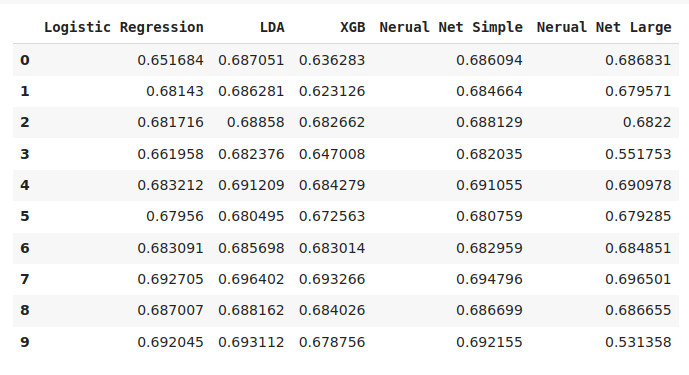
Fig 9: The accuracy of our models trying to predict changes in the moving average,

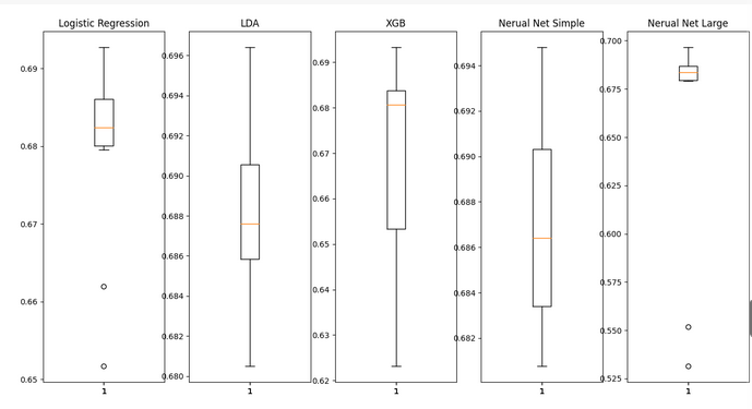
Fig 10: A visualization of our model's accuracy when forecasting changes in the moving average.

We will asses the highest accuracy recorded by each model type.

for i in enumerate(np.arrange(0,error_ma_df.shape[1])):
  print(error_ma_df.columns[i[0]]," ", error_ma_df.iloc[:,i[0]].max())

Logistic Regression   0.6927054112625546
LDA   0.696401658911147
XGB   0.6932664488520731
Neural Net Simple   0.6947955513019373
Neural Net Large   0.6965006655445914

Note that even though the large neural network attained the highest accuracy level outright, we would not wish to employ it in production because its performance was unstable. We can observe this from the 2 dots in the plot of the large neural network's performance that are far below its average performance. Therefore, we can observe from the results that given our current dataset, the ideal model should be more complex than a simple logistic regression and less complicated than a large neural network.

We will proceed onward by building a trading strategy that forecasts future movements in the moving average indicator as a trading signal. Our model of choice will be the small neural network because it appears a lot more stable.

We first import the libraries we need.

#Import the libraries we need
import MetaTrader5 as mt5
import pandas_ta as ta
import pandas as pd

Next, we setup our trading environment.

#Trading global variables
MARKET_SYMBOL = 'Volatility 75 Index'

#This data frame will store the most recent price update
last_close = pd.DataFrame()

#We may not always enter at the price we want, how much deviation can we tolerate?
DEVIATION = 10000

#We will always enter at the minimum volume
VOLUME = 0
#How many times the minimum volume should our positions be
LOT_MUTLIPLE = 1

#What timeframe are we working on?
TIMEFRAME = mt5.TIMEFRAME_M1

#Which model have we decided to work with?
neural_network_model= MLPClassifier(solver='lbfgs',alpha=1e-5,hidden_layer_sizes=(5, 2), random_state=1)

Let us determine the minimum volume allowed on the symbol we wish to trade.

#Determine the minimum volume
for index,symbol in enumerate(symbols):
    if symbol.name == MARKET_SYMBOL:
        print(f"{symbol.name} has minimum volume: {symbol.volume_min}")
        VOLUME = symbol.volume_min * LOT_MULTIPLE

We can now create a function that will deliver our market orders for us.

# function to send a market order
def market_order(symbol, volume, order_type, **kwargs):
    #Fetching the current bid and ask prices
    tick = mt5.symbol_info_tick(symbol)
    
    #Creating a dictionary to keep track of order direction
    order_dict = {'buy': 0, 'sell': 1}
    price_dict = {'buy': tick.ask, 'sell': tick.bid}

    request = {
        "action": mt5.TRADE_ACTION_DEAL,
        "symbol": symbol,
        "volume": volume,
        "type": order_dict[order_type],
        "price": price_dict[order_type],
        "deviation": DEVIATION,
        "magic": 100,
        "comment": "Indicator Forecast Market Order",
        "type_time": mt5.ORDER_TIME_GTC,
        "type_filling": mt5.ORDER_FILLING_FOK,
    }

    order_result = mt5.order_send(request)
    print(order_result)
    return order_result

Additionally, we also need another function that will help us close our market orders.

# Closing our order based on ticket id
def close_order(ticket):
    positions = mt5.positions_get()

    for pos in positions:
        tick = mt5.symbol_info_tick(pos.symbol) #validating that the order is for this symbol
        type_dict = {0: 1, 1: 0}  # 0 represents buy, 1 represents sell - inverting order_type to close the position
        price_dict = {0: tick.ask, 1: tick.bid} #bid ask prices

        if pos.ticket == ticket:
            request = {
                "action": mt5.TRADE_ACTION_DEAL,
                "position": pos.ticket,
                "symbol": pos.symbol,
                "volume": pos.volume,
                "type": type_dict[pos.type],
                "price": price_dict[pos.type],
                "deviation": DEVIATION,
                "magic": 10000,
                "comment": "Indicator Forecast Market Order",
                "type_time": mt5.ORDER_TIME_GTC,
                "type_filling": mt5.ORDER_FILLING_FOK,
            }

            order_result = mt5.order_send(request)
            print(order_result)
            return order_result

    return 'Ticket does not exist'

Furthermore, we must define the date range from which we want to request data.

#Update our date from and date to
date_from = datetime(2024,1,1)
date_to = datetime.now()

Before we can pass on the data requested from the broker, we must first preprocess the data into a the same format our model observed during training.

#Let's create a function to preprocess our data
def preprocess(df):
    #Calculating 60 period Simple Moving Average
    df.ta.sma(length=60,append=True)
    #Drop any rows that have missing values
    df.dropna(axis=0,inplace=True)

Moving on, we must be able to obtain a forecast from our neural network, and interpret that forecast as a trading signal to go long or short.

#Get signals from our model
def ai_signal():
    #Fetch OHLC data
    df = pd.DataFrame(mt5.copy_rates_range(market_symbol,TIMEFRAME,date_from,date_to))
    #Process the data
    df['time'] = pd.to_datetime(df['time'],unit='s')
    df['target'] = (df['close'].shift(-1) > df['close']).astype(int)
    preprocess(df)
    #Select the last row
    last_close = df.iloc[-1:,1:]
    #Remove the target column
    last_close.pop('target')
    #Use the last row to generate a forecast from our moving average forecast model
    #Remember 1 means buy and 0 means sell
    forecast = neural_network_model.predict(last_close)
    return forecast[0]

Finally we tie all this together to create our trading strategy.

#Now we define the main body of our trading algorithm
if __name__ == '__main__':
    #We'll use an infinite loop to keep the program running
    while True:
        #Fetching model prediction
        signal = ai_signal()
        
        #Decoding model prediction into an action
        if signal == 1:
            direction = 'buy'
        elif signal == 0:
            direction = 'sell'
        
        print(f'AI Forecast: {direction}')
        
        #Opening A Buy Trade
        #But first we need to ensure there are no opposite trades open on the same symbol
        if direction == 'buy':
            #Close any sell positions
            for pos in mt5.positions_get():
                if pos.type == 1:
                    #This is an open sell order, and we need to close it
                    close_order(pos.ticket)
            
            if not mt5.positions_totoal():
                #We have no open positions
                market_order(MARKET_SYMBOL,VOLUME,direction)
        
        #Opening A Sell Trade
        elif direction == 'sell':
            #Close any buy positions
            for pos in mt5.positions_get():
                if pos.type == 0:
                    #This is an open buy order, and we need to close it
                    close_order(pos.ticket)
            
            if not mt5.positions_get():
                #We have no open positions
                market_order(MARKET_SYMBOL,VOLUME,direction)
        
        print('time: ', datetime.now())
        print('-------\n')
        time.sleep(60)

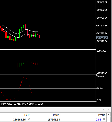
Fig 11: Our model in action.

Theoretical Explanation

In the writer's opinion, one of the reasons why we may be observing better accuracy when forecasting changes in technical indicators would have to be the fact we can never observe all the variables that are affecting the price of a security. At best, we can only observe them partially, whereas when forecasting the changes of a technical indicator, we are fully aware of all the inputs that have influenced the technical indicator. Recall that we even know the precise formula of any technical indicator.

Fig 12: We know the mathematical description of all technical indicators, but there is no mathematical formula of the close price.

For example, the Money Flow Multiplier (MFM) technical indicator is calculated using the formula above. Therefore, if we want to predict changes in the MFM, we only need the components of its formula: the close, low, and high prices.

In contrast, when forecasting the close price, we don't have a specific formula that tells us which inputs affect it. This often results in lower accuracy, suggesting that our current set of inputs may not be informative, or we have introduced too much noise by picking poor inputs.

Fundamentally speaking, the objective of machine learning is to find a target determined by a set of inputs. When we use a technical indicator as our target, we are essentially stating that the technical indicator is influenced by the open, close, low, and high prices, which is true. However, as algorithmic developers, we often use our tools the other way around. We use a collection of price data and technical indicators to forecast the price, implying that technical indicators influence the price, which is not the case and will never be the case.

When attempting to learn a target whose underlying function is not known, we potentially fall victim to what is known as a spurious regression, we discussed this at length in our previous discussion. In simple terms, it is possible for your model to learn a relationship that doesn't exist in real life. Furthermore, this flaw can be masked by deceptively low error rates upon validation making it appear as if the model has learned sufficiently, though in truth it hasn't learned anything about the real world.

To illustrate what a spurious regression is, imagine you and I were walking down a hill and just over the horizon we can see a vague shape. We are too far away to make out what it is, but based on what I've seen, I yell out "there's a dog down there". Now, upon arrival we find a bush, but behind the bush is a dog.

Fig 13: Could I have seen the dog?

Can you see the problem already? I would obviously love to claim the victory as a testimony of my perfect 20/20 vision, but you know that fundamentally speaking there was no possible way I could've seen the dog from where we stood when I made the statement, we were simply too far and the figure was too vague from where we stood.

There was simply no relationship between the inputs I saw at the top of the mountain and the conclusion I arrived at. That is to say, the input data and output data were independent of each other. Whenever a model looks at input data that has no relationship to the output data but manages to produce the right answer, we call that a spurious regression. Spurious regressions happen all the time!

Because we don't have technical formulas outlining what affects the price of a security, we are prone to making spurious regressions using inputs that have no influence over our target, being the close price. Trying to prove a regression isn't spurious can be challenging, it is easier to use a target that has a known relationship to the inputs.

Conclusion

This article has demonstrated why the practice of forecasting close price directly should potentially be deprecated in favor of forecasting changes in technical indicators instead. Further research is necessary to find out if there are any other technical indicators we can forecast with more accuracy than the moving average. However, readers should also be cautioned that while our accuracy of forecasting the moving average is relatively high, there is still a lag between the changes of the moving average and the changes in price.

In other words, it is possible for the moving average to be falling whilst price is rising, however if we as the MQL5 community collectively work to improve this algorithm, then I am confident that we may eventually reach new levels of accuracy.