Reimagining Classic Strategies (Part II): Bollinger Bands Breakouts

Introduction

Bollinger Bands are versatile tools in trading strategies, effective for both trend following and identifying potential turning or reversal points. Technically, the indicator is made up from an exponential moving average (EMA) that smooths out the closing price of a security. This central line is enveloped by two additional lines, positioned above and below the EMA by typically 2 standard deviations.

In this article, we aim to empirically analyze the benefits of strategy from the ground up.We aim to help readers who may be considering using the Bollinger Bands to decide whether the strategy may be better suited for them. Furthermore, we will show how technical indicators may be used to guide AI models and hopefully develop more stable trading strategies.

We achieved this by training two equivalent AI models using the Linear Discriminant Analysis algorithm and compared the models using time series cross-validation, relying solely on the scikit-learn library for the tests. The first model was trained to predict simply whether price would appreciate or depreciate, while the latter learned to forecast how the price moves between the four zones outlined by the Bollinger Band. Unfortunately for fans of Bollinger Bands, our empirical observations led us to conclude that predicting price directly may be more effective than forecasting the transition between the four zones created by the Bollinger Bands. However, it is worth noting that no optimization techniques were employed to set the parameters of the indicator.

This article aims to demonstrate:

1. How analytically compare two possible trading strategies.
   
2. How to implement Linear Discriminant Analysis from scratch in MQL5.
3. How to build stable trading strategies that incorporate AI.

Overview of the Strategy and Our Motivations

The term "Artificial Intelligence" (AI) is arguably one of the most misleading naming conventions in history. After reading this article, you may agree that AI is a misnomer. As the writer, my issue lies in the word "intelligence." AI models are not intelligent in the human sense. Instead, they are intelligent applications of optimization algorithms.

AI models primarily aim to minimize errors or maximize rewards within a system. However, solutions derived from these models may not always be practical. For example, an AI system designed to minimize losses in a trading account might conclude that placing no trades is the best solution, as it guarantees no losses. While mathematically satisfying the problem at hand, this solution is impractical for trading.

As intelligent AI practitioners, we must guide our models with carefully planned constraints. In this article, we will direct our AI models using Bollinger Bands. We will identify four possible zones where the price might be at any moment. Note that the price can only be in one of these four zones at any given time:

• Zone 1: Price is completely above the Bollinger Bands
• Zone 2: Price is above the mid-band but below the high-band
• Zone 3: Price is above the low-band but below the mid-band
• Zone 4: Price is below the low-band

We will train a model to understand how the price transitions between these four zones and predict the next zone the price will move to. Trading signals are generated whenever the price shifts from one zone to another. For instance, if our model predicts that the price will move from Zone 2 to Zone 1, we interpret this as an upward movement and initiate a buy order. Our model and Expert Advisor will be fully implemented in native MQL5.

Bollinger Bands can be utilized in a range of trading strategies, from trend following to identifying turning or reversal points. Technically, this indicator consists of an exponential moving average (EMA) that typically smooths out the close price of a security. It is flanked by two additional bands: one positioned above and one below the EMA, each normally set at 2 standard deviations.

Traditionally, Bollinger Bands are used to identify overbought and oversold price levels. When prices reach the upper Bollinger Band, they tend to fall back to the median value, and this behavior often holds true for the lower band as well. This can be interpreted as the security being discounted by 2 standard deviations when it hits the lower band, potentially attracting investors to buy the asset at an attractive discount. However, there are times when prices may break violently outside the Bollinger Bands and continue in a strong trend. Unfortunately, our statistical analysis shows that it may be more challenging to forecast Bollinger Band break-outs, than it is to forecast changes in price.

Fetching The Data From Our MetaTrader 5 Terminal

To begin, open up your MetaTrader5 terminal, and click on the Symbol icon in the context menu, you should see a list of symbols available on your terminal.

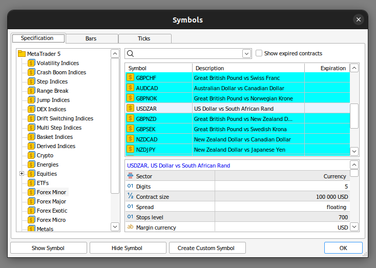
Fig 1: Preparing to fetch data from our MetaTrader5 Terminal.

Then click on the Bars window and search for the Symbol you'd like to model, select the time frame you wish to use. For our example I'll be modelling the GBPUSD Daily exchange rate.

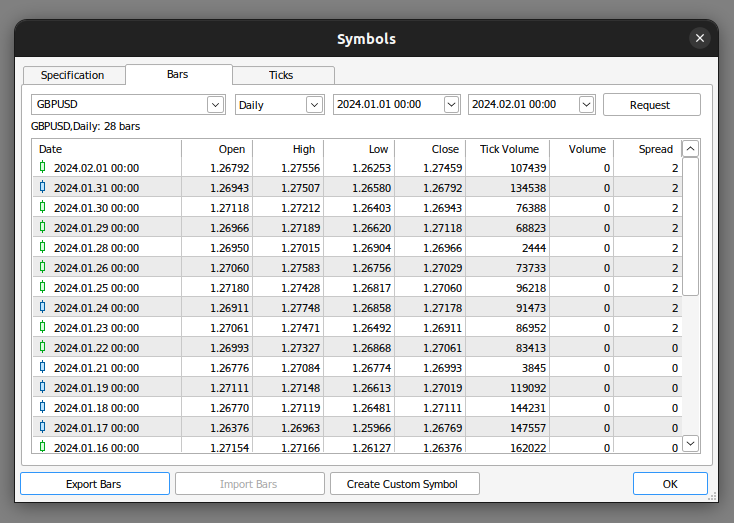
Fig 2: Preparing to export our data.

Then click the "Export Bars" button, and we will now continue our analysis in Python.

Exploratory Data Analysis

Let us visualize the interactions between the Bollinger Bands and the changes in price levels.

We will start off by importing the libraries we need.

#Import libraries
import pandas as pd
import numpy as np
import seaborn as sns
import pandas_ta as ta

Then we will read in the csv file we generated for our empirical test. Notice that we passed the parameter sep="\t" to denote that our csv file is tab delimited. This is the standard output from the MetaTrader5 Terminal.

#Read in the csv file
csv = pd.read_csv("/home/volatily/market_data/GBPUSD_Daily_20160103_20240131.csv",sep="\t")

Let us now define our forecast horizon.

#Define how far into the future we should forecast
look_ahead = 20

Now we will calculate the Bollinger Bands for the data we have using the pandas ta library.

#Add the Bollinger bands
csv.ta.bbands(length=30,std=2,append=True)

Next we need a column to store the future close price.

#Add a column to show the future price
csv["Future Close"] = csv["Close"].shift(-look_ahead)

Now we will label our data. We will have two labels, one denoting the change in price and the other denoting the change in price between the Bollinger Band zones. Changes in price will be labeled 1 for up, and 0 for down. The Bollinger Band labels were defined above.

#Add the normal target, predicting changes in the close price
csv["Price Target"] = 0
csv["Price State"] = 0
#Label the data our conditions
#If price depreciated, our label is 0 
csv.loc[csv["Close"] < csv["Close"].shift(look_ahead),"Price State"] = 0
csv.loc[csv["Close"] > csv["Future Close"], "Price Target"] = 0
#If price appreciated, our label is 1
csv.loc[csv["Close"] > csv["Close"].shift(look_ahead),"Price State"] = 1
csv.loc[csv["Close"] < csv["Future Close"], "Price Target"] = 1

#Label the Bollinger bands
#The label to store the current state of the market
csv["Current State"] = -1
#If price is above the upper-band, our label is 1
csv.loc[csv["Close"] > csv["BBU_30_2.0"], "Current State"] = 1
#If price is below the upper-band and still above the mid-band,our label is 2
csv.loc[(csv["Close"] < csv["BBU_30_2.0"]) & (csv["Close"] > csv["BBM_30_2.0"]),"Current State"] = 2
#If price is below the mid-band and still above the low-band,our label is 3
csv.loc[(csv["Close"] < csv["BBM_30_2.0"]) & (csv["Close"] > csv["BBL_30_2.0"]),"Current State"] = 3
#Finally, if price is beneath the low-band our label is 4
csv.loc[csv["Close"] < csv["BBL_30_2.0"], "Current State"] = 4
#Now we can add a column to denote the future state the market will be in
csv["State Target"] = csv["Current State"].shift(-look_ahead)

Let us delete any null entries.

#Let's drop any NaN values 
csv.dropna(inplace=True)

We are now ready to start visualizing our data, beginning with changes in price levels using box plots. On the y-axis, we will display the closing prices, and on the x-axis, we will have two values. The first value on the x-axis represents instances in our data where the price was falling, marked as 0. Within the 0 value, you will observe two box plots. The first box plot, shown in blue, represents instances where the price fell for 20 candles and continued falling for another 20 candles. The orange box plot represents instances where the price fell for 20 candles but then appreciated over the next 20 candles. Notice that in the data we collected, it appears that whenever price levels fell below 1.1, they always rebounded. Conversely, the 1 value on the x-axis also has two box plots above it. The first blue box plot summarizes instances where the price appreciated and then depreciated, while the second orange box plot summarizes instances where the price rose and continued rising.

Notice that for the 1 value, or in other words when price rises for 20 candles, the tail of the blue box plot is greater than that of the orange box plot. This may indicate that whenever the GBPUSD exchange rate rises towards the 1.5 level, it tends to fall, whereas on the 0 column, when the exchange rate fall to around the 1.1 level, it appears that price has a tendency to reverse and start rising.

#Notice that the tails of the box plots have regions where they stop overlapping these zones may guide us as boundaries
sns.boxplot(data=csv,x="Price State",y="Close",hue="Price Target")

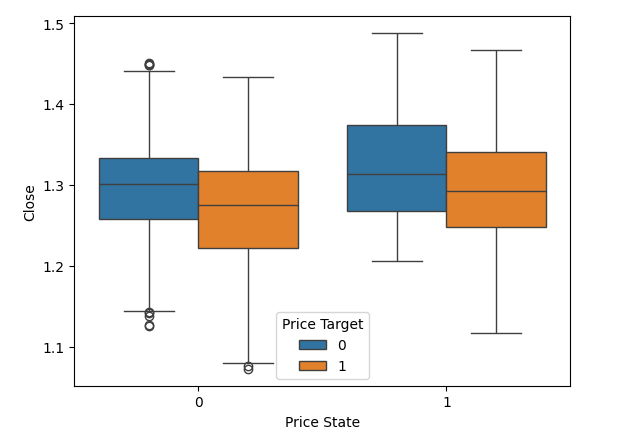
Fig 3: Visualizing the changes in price levels.

We can also perform similar visualizations using the states defined by the Bollinger Bands. As before, the closing price will be on the y-axis, and the current location of the price within the Bollinger Bands will be marked by the four values on the x-axis. Notice that the tails of the box plots have regions where they naturally do not overlap. These regions may potentially serve as classification boundaries. For example, observe that whenever the price is in state 4, or completely beneath the Bollinger Bands, and it approaches the 1.1 level, it appears to always rebound.

#Notice that the tails of the box plots have regions where they stop overlapping these zones may guide us as boundaries
sns.boxplot(data=csv,x="Current State",y="Close",hue="Price Target")

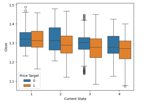
Fig 4: Visualizing the behavior of price within the 4 zones of the Bollinger Bands.

Moreover, we can also visualize how the price transitions between the four Bollinger Band states using box plots. For example, the box plot below has the closing price on the y-axis and four values on the x-axis denoting the four zones created by the Bollinger Bands. Each box plot summarizes where the price transitioned to after appearing in that zone. Let's interpret the data together. Notice that the first value, state 1, only has three box plots. This means that from state 1, the price only transitions to three possible states: it either remains in state 1 or transitions to states 2 or 3.

#Notice that the tails of the box plots have regions where they stop overlapping these zones may guide us as boundaries
sns.boxplot(data=csv,x="Current State",y="Close",hue="State Target")

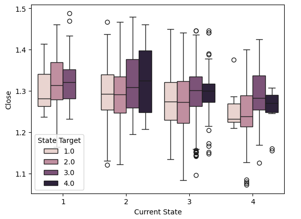
Fig 5: Visualizing the behavior of price within the 4 zones.

We will create a categorical plot with the closing price on the y-axis and two values on the x-axis. The first value, Price State 0, indicates instances where the price fell over the prior 10 candles. Above State 0, there is a cloud of blue and orange dots. These dots represent instances where, after falling for 10 candles, the price either continued falling or reversed and started rising for the next 10 candles, respectively. Notice that there is no clear separation between the instances where the price continued falling and where it turned around and started rising. It appears that the only well-defined separation point is when the price approaches extreme values. For example, at all price levels below 1.1 in State 0, the price consistently rebounded.

#we have very poor separation in the data
sns.catplot(data=csv,x="Price State",y="Close",hue="Price Target")

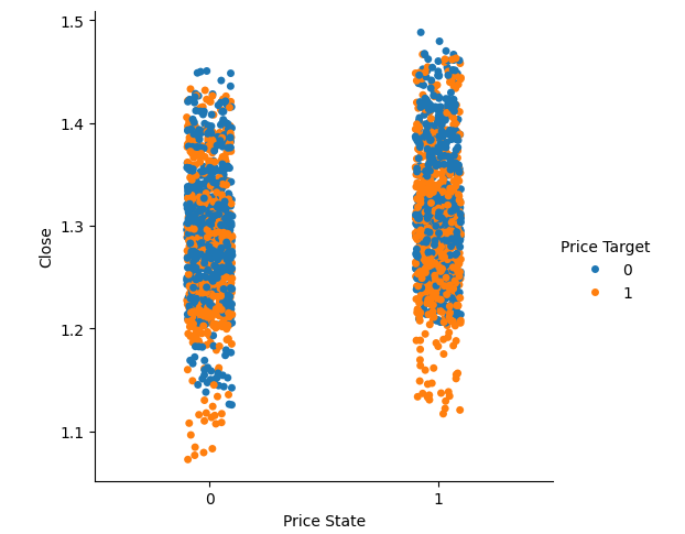
Fig 6: Visualizing the separation in the dataset.

We can perform the same visualizations using the four states defined by the Bollinger Bands. Once again, we observe that the blue and orange dots are best separated at the extreme price levels.

#Visualizing the separation of data in the Bollinger band zones
sns.catplot(data=csv,x="Current State",y="Close",hue="Price Target")

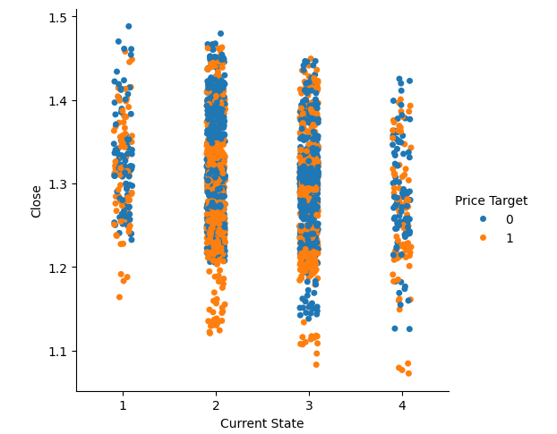
Fig 7:Visualizing the separation of data in the Bollinger Band zones.

We can now create a scatter plot with the closing value on the x-axis and the future closing price on the y-axis. We will color the dots either orange or blue depending on whether the price rose or fell over the previous 20 candles. Imagine placing a golden line from the bottom-left corner to the top-right corner of the plot. All points above this golden line represent instances where the price ended up rising over the next 20 candles, regardless of whether it fell (blue) or rose (orange) over the previous 20 candles. Notice that there is a mixture of blue and orange dots on both sides of the golden line.

Furthermore, observe that if we placed an imaginary red line at the closing value of 1.3, there would be many blue and orange dots touching this line. This implies that other variables affect the future closing price besides the current closing price. Another way to interpret these observations is that the same input value may result in different output values, indicating that our dataset is noisy!

#Notice that using the price target gives us beautiful separation in the data set
sns.scatterplot(data=csv,x="Close",y="Future Close",hue="Price Target")

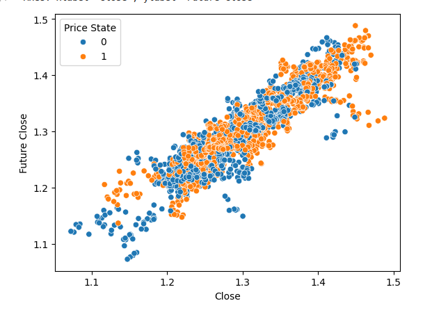
Fig 8: Our dataset has very little natural separation.

We will now perform the same visualization using the Bollinger Bands' target state to color the scatter plot. Notice that we have very poor separation within our dataset when using the Bollinger Bands. Visually, it appears even worse than the separation we obtained when we simply used the price itself.

#Using the Bollinger bands to define states, however, gives us rather mixed separation
sns.scatterplot(data=csv,x="Close",y="Future Close",hue="Current State")

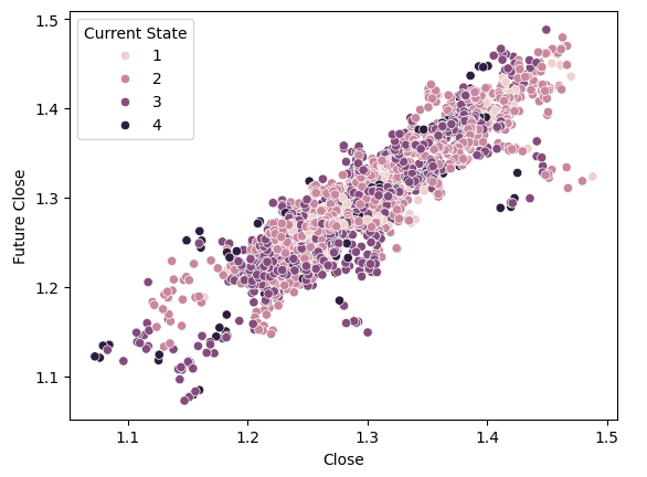
Fig 9: Visualizing the separation in the dataset created by the Bollinger Band Zones.

Let us now perform our analytical tests to determine whether we achieve greater accuracy in predicting changes in price levels or changes in Bollinger Band states. First, we import the necessary libraries.

#Now let us compare our accuracy forecasting the original price target and the new Bollinger bands target
from sklearn.discriminant_analysis import LinearDiscriminantAnalysis
from sklearn.model_selection import TimeSeriesSplit
from sklearn.metrics import accuracy_score

Next, we will define our time series cross-validation parameters. The first parameter, splits, specifies the number of partitions to create from our data. The second parameter, gap, determines the size of the gap between each partition. This gap should be at least as large as our forecast horizon.

#Now let us define the cross validation parameters
splits = 10
gap = look_ahead

Now we can create our time series object, which will provide us with the appropriate indexes for our training set and test set. In our example, it will generate 10 pairs of indexes to train and evaluate our model.

#Now create the cross validation object
tscv = TimeSeriesSplit(n_splits=splits,gap=gap)

Next, we will create a DataFrame to store the accuracy of our model for forecasting each target.

#We need a dataframe to store the accuracy associated with each target
target_accuracy = pd.DataFrame(index=np.arange(0,splits),columns=["Price Target Accuracy","New Target Accuracy"])

Now we will define our model inputs.

#Define the inputs
predictors = ["Open","High","Low","Close"]
target = "Price Target"

Now we will perform the cross-validation test.

#Now let us perform the cross validation
for i,(train,test) in enumerate(tscv.split(csv)):
    #First initialize the model
    model = LinearDiscriminantAnalysis()
    #Now train the model
    model.fit(csv.loc[train[0]:train[-1],predictors],csv.loc[train[0]:train[-1],target])
    #Now record the accuracy
    target_accuracy.iloc[i,0] = accuracy_score(csv.loc[test[0]:test[-1],target],model.predict(csv.loc[test[0]:test[-1],predictors]))

Now we can finally analyze the result of the tests.

target_accuracy

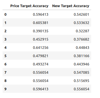
Fig 10: Our model performed better when forecasting changes in price directly.

As mentioned before, our tests showed that our model is more effective at predicting price levels than Bollinger Band transitions. However, note that, on average, the two strategies are not significantly different.

Next, we will implement the strategy in MQL5 code to back test it and see how it performs on real market data

Implementing The Strategy

To get started, we will first import the necessary libraries that we will use throughout our program.

//+------------------------------------------------------------------+
//|                                           Target Engineering.mq5 |
//|                                        Gamuchirai Zororo Ndawana |
//|                                             https://www.mql5.com |
//+------------------------------------------------------------------+
#property copyright "Gamuchirai Zororo Ndawana"
#property link      "https://www.mql5.com"
#property version   "1.00"
//+------------------------------------------------------------------+
//| Libraries we need                                                |
//+------------------------------------------------------------------+
/*
   This Expert Advisor will implement the Linear Discriminant Anlysis
   algorithm to help us successfully trade Bollinger Band Breakouts.

   Gamuchirai Zororo Ndawana
   Selebi Phikwe
   Botswana
   Wednesday 10 July 2024 15:42
*/
#include <Trade/Trade.mqh>//Trade class
CTrade Trade;

Next, we will define user-configurable inputs, such as the Bollinger Bands period and standard deviation.

//+------------------------------------------------------------------+
//| Input variables                                                  |
//+------------------------------------------------------------------+
input double bband_deviation = 2.0;//Bollinger Bands standard deviation
input int    bband_period = 60; //Bollinger Bands Period
input int look_ahead = 10; //How far into the future should we forecast?
int input  lot_multiple = 1; //How many times bigger than minimum lot?
int input    fetch = 200;//How much data should we fetch?
input double stop_loss_values = 1;//Stop loss values

Subsequently, we will define the global variables that will be used in our application.

//+------------------------------------------------------------------+
//| Global variables                                                 |
//+------------------------------------------------------------------+
int bband_handler;//Technical Indicator Handlers
vector bband_high_reading = vector::Ones(fetch);//Bollinger band high reading
vector bband_mid_reading = vector::Ones(fetch);//Bollinger band mid reading
vector bband_low_reading = vector::Ones(fetch);//Bollinger band low reading
double minimum_volume;//The smallest contract size allowed
double ask_price;//Ask
double bid_price;//Bid
vector input_data = vector::Zeros(fetch);//All our input data will be kept in vectors
int training_output_array[];//Our output data will be stored in a vector
vector output_data = vector::Zeros(fetch);
double variance;//This is the variance of our input data
int classes = 4;//The total number of output classes we have
vector mean_values = vector::Zeros(classes);//This vector will store the mean value for each class
vector probability_values = vector::Zeros(classes);//This vector will store the prior probability the target will belong each class
vector total_class_count = vector::Zeros(classes);//This vector will count the number of times each class was the target
bool model_trained = false;//Has our model been trained?
bool training_procedure_running = false;//Have we started the training process?
int forecast = 0;//Our model's forecast
double discriminant_values[4];//The discriminant function
int current_state = 0;//The current state of the system

Next, we need to define the initialization function of our Expert Advisor. In this function, we will initialize the Bollinger Bands indicator and fetch important market data.

//+------------------------------------------------------------------+
//| Expert initialization function                                   |
//+------------------------------------------------------------------+
int OnInit()
  {
//--- Initialize the bollinger bands
   bband_handler = iBands(_Symbol,PERIOD_CURRENT,bband_period,0,bband_deviation,PRICE_CLOSE);
//--- Market data
   minimum_volume = SymbolInfoDouble(_Symbol,SYMBOL_VOLUME_MIN);
//--- End of initilization
   return(INIT_SUCCEEDED);
  }

Following this, we will define essential helper functions to break our code into smaller, more manageable segments. The first function we will create will be responsible for updating our market data.

//+------------------------------------------------------------------+
//|This function will update the price and other technical data      |
//+------------------------------------------------------------------+
void update_technical_data(void)
  {
//--- Update the bid and ask prices
   ask_price = SymbolInfoDouble(_Symbol,SYMBOL_ASK);
   bid_price = SymbolInfoDouble(_Symbol,SYMBOL_BID);
  }

Subsequently, we need to implement a function that orchestrates the initialization procedure. This function will ensure that we fetch training data, fit our model, and begin making forecasts in the correct sequence.

//+------------------------------------------------------------------+
//|This function will start training our model                       |
//+------------------------------------------------------------------+
void model_initialize(void)
  {
//--- First we have to fetch the input and output data
   Print("Initializing the model");
   int input_start = 1 + (look_ahead * 2);
   int output_start = 1+ look_ahead;
   fetch_input_data(input_start,fetch);
   fetch_output_data(output_start,fetch);
//--- Fit the model
   fit_lda_model();
  }

Following this, we will define the function responsible for fetching input data to train our model. It's important to note that the model's input will consist of the current state of the market—specifically, which zone the market currently occupies. The model will then forecast which zone the market will move to next.

//+------------------------------------------------------------------+
//|This function will fetch the inputs for our model                 |
//+------------------------------------------------------------------+
void fetch_input_data(int f_start,int f_fetch)
  {
//--- This function will fetch input data for our model   Print("Fetching input data");
//--- The input for our model will be the current state of the market
//--- To know the current state of the market, we have to first update our indicator readings
   bband_mid_reading.CopyIndicatorBuffer(bband_handler,0,f_start,f_fetch);
   bband_high_reading.CopyIndicatorBuffer(bband_handler,1,f_start,f_fetch);
   bband_low_reading.CopyIndicatorBuffer(bband_handler,2,f_start,f_fetch);
   vector historical_prices;
   historical_prices.CopyRates(_Symbol,PERIOD_CURRENT,COPY_RATES_CLOSE,f_start,f_fetch);
//--- Reshape the input data
   input_data.Resize(f_fetch);
//--- Now we will input the state of the market
   for(int i = 0; i < f_fetch;i++)
     {
      //--- Are we above the bollinger bands entirely?
      if(historical_prices[i] > bband_high_reading[i])
        {
         input_data[i] = 1;
        }

      //--- Are we between the upper and mid band?
      else
         if((historical_prices[i]  < bband_high_reading[i]) && (historical_prices[i] > bband_mid_reading[i]))
           {
            input_data[i] = 2;
           }

         //--- Are we between the mid and lower band?
         else
            if((historical_prices[i]  < bband_mid_reading[i]) && (historical_prices[i]  > bband_low_reading[i]))
              {
               input_data[i] = 3;
              }

            //--- Are we below the bollinger bands entirely?
            else
               if(historical_prices[i]  < bband_low_reading[i])
                 {
                  input_data[i] = 4;
                 }
     }
//--- Show the input data
   Print(input_data);
  }

Moving forward, we require a function to retrieve the output data for our model. This task is more intricate than fetching the input data. We must not only record the final zone that the price ended in but also track how many times each zone was the output. This count is crucial for estimating the parameters of our LDA model at a later stage.

From this point onward, we are prepared to fit our LDA model. There are various methods available for fitting the model; today, we will focus on one specific approach.

//+---------------------------------------------------------------------+
//|Fetch the output data for our model                                  |
//+---------------------------------------------------------------------+
void fetch_output_data(int f_start,int f_fetch)
  {
//--- The output for our model will be the state of the market
//--- To know the state of the market, we have to first update our indicator readings
   Print("Fetching output data");
   bband_mid_reading.CopyIndicatorBuffer(bband_handler,0,f_start,(f_fetch));
   bband_high_reading.CopyIndicatorBuffer(bband_handler,1,f_start,(f_fetch));
   bband_low_reading.CopyIndicatorBuffer(bband_handler,2,f_start,(f_fetch));
   vector historical_prices;
   historical_prices.CopyRates(_Symbol,PERIOD_CURRENT,COPY_RATES_CLOSE,f_start,f_fetch);
//--- First we have to ensure that the class count has been reset
   total_class_count[0] = 0;
   total_class_count[1] = 0;
   total_class_count[2] = 0;
   total_class_count[3] = 0;
//--- Now we need to resize the matrix
   ArrayResize(training_output_array,f_fetch);
//--- Now we will input the state of the market to our output vector
   for(int i =0 ; i < f_fetch;i++)
     {
      //--- Are we above the bollinger bands entirely?
      if(historical_prices[i] > bband_high_reading[i])
        {
         training_output_array[i] = 1;
         total_class_count[0] += 1;
        }

      //--- Are we between the upper and mid band?
      else
         if((historical_prices[i] < bband_high_reading[i]) && (historical_prices[i] > bband_mid_reading[i]))
           {
            training_output_array[i] = 2;
            total_class_count[1] += 1;
           }

         //--- Are we between the mid and lower band?
         else
            if((historical_prices[i] < bband_mid_reading[i]) && (historical_prices[i] > bband_low_reading[i]))
              {
               training_output_array[i] = 3;
               total_class_count[2] += 1;
              }

            //--- Are we below the bollinger bands entirely?
            else
               if(historical_prices[i] < bband_low_reading[i])
                 {
                  training_output_array[i] = 4;
                  total_class_count[3] += 1;
                 }
     }
//--- Show the output data
   Print("Final state of output vector");
   ArrayPrint(training_output_array);
//--- Show the total number of times each class appeared as the target.
   Print(total_class_count);
  }

The process is a bit intricate and requires detailed explanation. Initially, we calculate the total sum of all input values corresponding to each class in the output. For instance, for every instance where the target was 1, we compute the sum of all input values mapped to an output of 1, and so forth for each output class.  Subsequently, we compute the mean value of X for each class. If there were multiple inputs, we would calculate the mean value for each input. Moving forward, we proceed to determine the probability of each class appearing as the actual target, based on the training set data. Following that, we compute the variance of X for each class of y.  Finally, we update our flags to indicate the completion of the training procedure.

//+------------------------------------------------------------------+
//|Fit the LDA model                                                 |
//+------------------------------------------------------------------+
void fit_lda_model(void)
  {

//--- To fit the LDA model, we first need to know the mean value for each our inputs for each of our 4 classes
   double sum_class_one = 0;
   double sum_class_two = 0;
   double sum_class_three = 0;
   double sum_class_four = 0;

//--- In this case we only have 1 input
   for(int i = 0; i < fetch;i++)
     {
      //--- Class 1
      if(training_output_array[i] == 1)
        {
         sum_class_one += input_data[i];
        }
      //--- Class 2
      else
         if(training_output_array[i] == 2)
           {
            sum_class_two += input_data[i];
           }
         //--- Class 3
         else
            if(training_output_array[i] == 3)
              {
               sum_class_three += input_data[i];
              }
            //--- Class 4
            else
               if(training_output_array[i] == 4)
                 {
                  sum_class_four += input_data[i];
                 }
     }
//--- Show the sums
   Print("Class 1: ",sum_class_one," Class 2: ",sum_class_two," Class 3: ",sum_class_three," Class 4: ",sum_class_four);
//--- Calculate the mean value for each class
   mean_values[0] = sum_class_one / fetch;
   mean_values[1] = sum_class_two / fetch;
   mean_values[2] = sum_class_three / fetch;
   mean_values[3] = sum_class_four / fetch;
   Print("Mean values");
   Print(mean_values);
//--- Now we need to calculate class probabilities
   for(int i=0;i<classes;i++)
     {
      probability_values[i] = total_class_count[i] / fetch;
     }
   Print("Class probability values");
   Print(probability_values);
//--- Calculating the variance
   Print("Calculating the variance");
//--- Next we need to calculate the variance of the inputs within each class of y.
//--- This process can be simplified into 2 steps
//--- First we calculate the difference of each instance of x from the group mean.
   double squared_difference[4];
   for(int i =0; i < fetch;i++)
     {
      //--- If the output value was 1, find the input value that created the output
      //--- Calculate how far that value is from it's group mean and square the difference
      if(training_output_array[i] == 1)
        {
         squared_difference[0] = MathPow((input_data[i]-mean_values[0]),2);
        }

      else
         if(training_output_array[i] == 2)
           {
            squared_difference[1] = MathPow((input_data[i]-mean_values[1]),2);
           }

         else
            if(training_output_array[i] == 3)
              {
               squared_difference[2] = MathPow((input_data[i]-mean_values[2]),2);
              }

            else
               if(training_output_array[i] == 4)
                 {
                  squared_difference[3] = MathPow((input_data[i]-mean_values[3]),2);
                 }
     }

//--- Show the squared difference values
   Print("Squared difference value for each output value of y");
   ArrayPrint(squared_difference);

//--- Next we calculate the variance as the average squared difference from the mean
   variance = (1.0/(fetch - 4.0)) * (squared_difference[0] + squared_difference[1] + squared_difference[2] + squared_difference[3]);
   Print("Variance: ",variance);

//--- Update our flags to denote the model has been trained
   model_trained = true;
   training_procedure_running = false;
  }
//+------------------------------------------------------------------+

To make a forecast with our model, we begin by fetching the latest input data from the market. Using this input data, we calculate the discriminant function for each possible class. The class with the highest discriminant function value will be our predicted class.

In MQL5, arrays offer a useful function called ArrayMaximum() which returns the index of the largest value in a 1D array. Since arrays are zero-indexed, we add 1 to the result of ArrayMaximum() to obtain the predicted class.

//+------------------------------------------------------------------+
//|This function will obtain forecasts from our model                |
//+------------------------------------------------------------------+
int model_forecast(void)
  {
//--- First we need to fetch the most recent input data
   fetch_input_data(0,1);
//--- Update the current state of the system
   current_state = input_data[0];

//--- We need to calculate the discriminant function for each class
//--- The predicted class is the one with the largest discriminant function
   Print("Calculating discriminant values.");
   for(int i = 0; i < classes; i++)
     {
      discriminant_values[i] = (input_data[0] * (mean_values[i]/variance) - (MathPow(mean_values[i],2)/(2*variance)) + (MathLog(probability_values[i])));
     }

   ArrayPrint(discriminant_values);
   return(ArrayMaximum(discriminant_values) + 1);
  }

After obtaining a forecast from our model, the next step is to interpret it and decide accordingly. As mentioned earlier, our trading signals are generated when the model predicts that the price will move to a different zone:

1. If the forecast indicates a move from zone 1 to zone 2, this triggers a sell signal.
2. Conversely, a forecast of moving from zone 4 to zone 3 indicates a buy signal.
3. However, if the forecast suggests that the price will remain in the same zone (e.g., from zone 1 to zone 1), this does not generate an entry signal.

//+--------------------------------------------------------------------+
//|This function will interpret out model's forecast and execute trades|
//+--------------------------------------------------------------------+
void find_entry(void)
  {
//--- If the model's forecast is not equal to the current state then we are interested
//--- Otherwise whenever the model forecasts that the state will remain the same
//--- We are uncertain whether price levels will rise or fall
   if(forecast != current_state)
     {
      //--- If the model forecasts that we will move from a small state to a greater state
      //--- That is from 1 to 2 or from 2 to 4 then that is a down move
      if(forecast > current_state)
        {
         Trade.Sell(minimum_volume * lot_multiple,_Symbol,bid_price,(bid_price + stop_loss_values),(bid_price - stop_loss_values));
        }

      //--- Otherwise we have a buy setup
      else
        {
         Trade.Buy(minimum_volume * lot_multiple,_Symbol,ask_price,(ask_price - stop_loss_values),(ask_price +stop_loss_values));
        }
     }
//--- Otherwise we do not have an entry signal from our model
  }

Finally, our OnTick() event handler is responsible for managing event flow and ensuring that we only trade when our model has been trained, along with satisfying our other trading conditions.

//+------------------------------------------------------------------+
//| Expert tick function                                             |
//+------------------------------------------------------------------+
void OnTick()
  {
//--- We must always update market data
   update_technical_data();
//--- First we must ensure our model has been trained
   switch(model_trained)
     {

      //--- Our model has been trained
      case(true):
         //--- If we have no open positions, let's obtain a forecast from our model
         if(PositionsTotal() == 0)
           {
            //--- Obtaining a forecast
            forecast = model_forecast();
            Comment("Model forecast: ",forecast);
            //--- Find an entry setup
            find_entry();
           }
         break;
      //--- End of case 1

      //--- Our model has not been trained
      default:
         //--- We haven't started the training procedure!
         if(!training_procedure_running)
           {
            Print("Our model has not been trained, starting the training procedure now.");
            //--- Initialize the model
            model_initialize();
           }

         break;
         //--- End of default case
     }
  }
//+------------------------------------------------------------------+

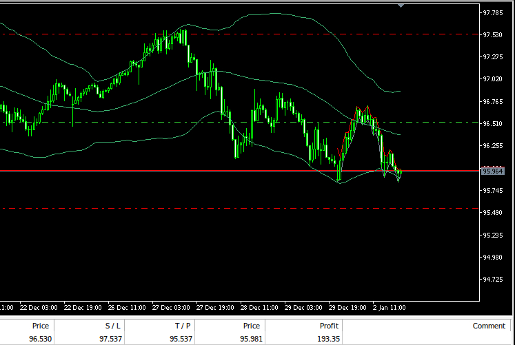
Fig 11: Our trading system in action.

Limitations

Up to this point, our strategy faces a significant limitation: it can be challenging to interpret. When our model predicts that the price will stay in the same zone, we lack clarity on whether prices will rise or fall. This trade-off stems from our decision to categorize market states into four distinct zones, which enhances accuracy but sacrifices transparency compared to directly forecasting price movements. Additionally, this approach generates fewer trading signals because we must wait for the model to predict a zone change before taking action.

Conclusion

In conclusion, our strategy harnesses the power of machine learning, specifically Linear Discriminant Analysis (LDA), integrated with Bollinger Bands for trading signals. While providing enhanced accuracy, our approach sacrifices some transparency. All in all traders may be better off forecasting changes in price than they are forecasting Bollinger Band breakouts.