
Neural networks made easy (Part 73): AutoBots for predicting price movements

Introduction
Effectively predicting the movement of currency pairs is a key aspect of secure trading management. In this context, special attention is paid to developing efficient models that can accurately approximate the joint distribution of contextual and temporal information required for making trading decisions. As a possible solution to such tasks, let's discuss a new method called "Latent Variable Sequential Set Transformers" (AutoBots) presented in the paper "Latent Variable Sequential Set Transformers For Joint Multi-Agent Motion Prediction". The proposed method is based on the Encoder-Decoder architecture. It was developed to solve problems of safe control of robotic systems. It allows the generation of sequences of trajectories for multiple agents consistent with the scene. AutoBots can predict the trajectory of one ego-agent or the distribution of future trajectories for all agents in the scene. In our case, we will try to apply the proposed model to generate sequences of price movements of currency pairs consistent with market dynamics.
1. AutoBots algorithms
"Latent Variable Sequential Set Transformers" (AutoBots) is a method based on the Encoder-Decoder architecture. It processes sequences of sets. AutoBot is fed with a sequence of sets X1:t = (X1, …, Xt), which in the problem of predicting movement can be considered as the environment state for t time steps. Each set contains M elements (agents, financial instruments and/or indicators) with K attributes (signs). To process social and temporal information in the Encoder, the following two transformations are used.
First, the AutoBots Encoder introduces temporal information into a sequence of sets using a sine positional encoding function PE(.). At this stage, the data is analyzed as a collection of matrices, {X0, …, XM}, which describe the evolution of agents over time. The encoder processes temporal relationships between sets using a multi-head attention block.
This is followed by the processing of slices S by extracting sets of agent states Sꚍ at a certain moment of time ꚍ. They are processed again in the multi-headed attention block.
These two operations are repeated Lenc times to obtain a context tensor C of dimension {dK, M, t}, which summarizes the entire scene representation of the original data, where t is the number of time steps in the source data scene.
The goal of the Decoder is to generate predictions that are temporally and socially consistent in the context of multimodal data distributions. To generate c different forecasts or the same scene of the original data, the AutoBot Decoder uses c matrices of trainable initial parameters Qi having the dimension {dK, T}, where T is the planning horizon.
Intuitively, each matrix of trainable initial parameters corresponds to the setting of a discrete latent variable in AutoBot. Each trainable matrix Qi is then repeated M times along the agent dimension to obtain the input tensor Q0i having the dimension {dK, M, T}.
The algorithm provides the ability to use additional contextual information, which is encoded using a convolutional neural network to create a feature vector mi. To provide contextual information to all future time steps and all elements of the set, it is proposed to copy this vector along dimensions M and T, creating a tensor Mi with the dimension {dK, M, T}. Each tensor Q0i is then combined with Mi along dimension dK. This tensor is then processed using the fully connected layer (rFFN) to obtain the tensor H of dimension {dK, M, T}.
Decoding begins by processing the time dimension determined at the output of the Encoder (C), as well as encoded initial parameters and information about the environment (H). The decoder processes each agent in H separately, using a multi-headed attention block. Thus, we obtain a tensor that encodes the future time evolution of each element of the set independently.
To ensure social consistency of the future scene between elements of the set, we process each time slice H0, extracting sets of agent states H0ꚍ at some future point in time ꚍ. Each element of the sequence is processed by a multi-head attention unit. This block performs attention at each time step between all elements of the set.
These two operations are repeated Ldec times to create the final output tensor for the agent i. The decoding process is repeated c times with different trained initial parameters Qi and additional contextual information mi. The output of the decoder is tensor O with the dimension {dK, M, T, c}, which can then be processed using a neural network ф(.) to get the desired output representation.
One of the main contributions that makes the result and training time of AutoBot faster compared to other methods is the use of initial decoder parameters Qr. These options have a dual purpose. First, they take into account diversity in predicting the future, where each matrix Qi corresponds to one setting of a discrete latent variable. Second, they help speed up AutoBot by allowing it to infer across an entire scene with a single pass through the Decoder without sequential selection.
The original visualization of the method presented by the paper authors is provided below.
 method provided by the paper authors")
2. Implementation using MQL5
We have discussed the theoretical aspects of the Latent Variable Sequential Set Transformers (AutoBots) method. Now let's move on to the practical part of the article, in which we will implement our vision of the presented method using MQL5.
To begin with, you should pay attention to the following 2 points.
First, the method provides positional coding. However, we have already seen similar positional coding utilized within the basic Self-Attention method. But the fact is that earlier, when studying attention methods, positional coding of the source data was implemented on the side of the main program. However, in AutoBot, positional coding is implemented within the model after preliminary processing and creation of embedding of the source data. Of course, we could move the data preprocessing into a separate model and implement positional encoding on the side of the main program before transferring data to the Encoder. But this option would require additional data transfer operations between the memory of the OpenCL context and the main program. In addition, such an implementation would limit our flexibility in using various model architectures within a single program without making additional adjustments to its code. Therefore, a preferable way is to organize the entire process within one model.
Second, both in the Encoder and in the Decoder, the Latent Variable Sequential Set Transformers (AutoBots) method requires an alternative use of attention blocks within the framework of various dimensions of the analyzed tensors (analysis of time and social dependencies). To change the dimension of the attention focus, we need to modify the multi-headed attention layer CNeuronMLMHAttentionOCL or transpose tensors. Transposing tensors looks like a simpler task here. This requires certain steps which were previously discussed for positional coding. We will not repeat them here. It's just that we need to create a tensor transposition layer on the OpenCL context side.
2.1 Positional encoding layer
We'll start with the positional encoding layer. We inherit the positional encoding layer class CNeuronPositionEncoder from the neural layer base class of our CNeuronBaseOCL library and override the basic set of methods:
- Init — initialization
- feedForward — feed-forward pass
- calcInputGradients — error gradient propagation to the previous layer
- updateInputWeights — updating weights
- Save and Load — file operations
class CNeuronPositionEncoder  :  public CNeuronBaseOCL
  {
protected:
   CBufferFloat      PositionEncoder;

   virtual bool      feedForward(CNeuronBaseOCL *NeuronOCL);
   virtual bool      updateInputWeights(CNeuronBaseOCL *NeuronOCL)
                         { return true; }

public:
                     CNeuronPositionEncoder(void) {};
                    ~CNeuronPositionEncoder(void) {};
   //---
   virtual bool      Init(uint numOutputs, uint myIndex, COpenCLMy *open_cl, uint count, uint window, ENUM_OPTIMIZATION optimization_type, uint batch);
   virtual bool      calcInputGradients(CNeuronBaseOCL *NeuronOCL)
                         { return true; }
   //---
   virtual bool      Save(int const file_handle);
   virtual bool      Load(int const file_handle);
   //---
   virtual int       Type(void) const
                         { return defNeuronPEOCL; }
   virtual void      SetOpenCL(COpenCLMy *obj);
  };
We leave the constructor and destructor of the class empty.
Before we move on to other methods, let's discuss a little the class functionality and construction logic. In the Transformer algorithm, positional encoding is implemented by adding sinusoidal harmonics to source data using the following functions:
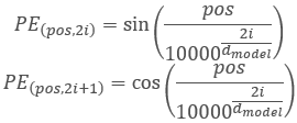
Please note that in this case, we perform positional encoding for the elements in the analyzed sequence. It is not associated with the timestamp harmonics used earlier, which we create on the side of the main program. The process is similar, but the meaning is different.
Obviously, the size of the analyzed sequence in the model will always be constant. Therefore, we can simply create and fill a harmonic buffer PositionEncoder in the class initialization method Init. During the feed-forward pass, in the feedForward method, we just add the harmonic values to the original data.
This concerns the feed-forward pass. What about the backpropagation pass? In the feed-forward pass, we performed the addition of two tensors. Consequently, the error gradient during the backpropagation pass is evenly distributed or completely transferred to both terms. The harmonic tensor of positional coding in our case is a constant. Therefore, we will transfer the entire error gradient to the previous layer.
As for trainable weights, they simply do not exist in the positional coding layer. Therefore, the updateInputWeights method is overridden only for class compatibility and always returns true.
This is the logic. Let's now look at the implementation. The class is initialized in the Init method. The method receives in parameters:
- numOutputs — number of connections to the next layer
- open_cl — pointer to OpenCL context
- count — number of elements in the sequence
- window — number of parameters for each element of the sequence
- optimization_type — parameter optimization method.
bool CNeuronPositionEncoder::Init(uint numOutputs, uint myIndex,
                                  COpenCLMy *open_cl, uint count,
                                  uint window,
                                  ENUM_OPTIMIZATION optimization_type,
                                  uint batch)
  {
   if(!CNeuronBaseOCL::Init(numOutputs, myIndex, open_cl, count * window,
                                                 optimization_type, batch))
      return false;
In the body of the method, we call the initialization method of the parent class, which implements the basic functionality. We also check the result of the operations.
Next we need to create position encoding harmonics. We will use matrix operations for this. First, let's prepare the matrix.
matrix<float> pe = matrix<float>::Zeros(count, window);
We create a vector for numbering the positions of elements in the tensor and a constant factor that is used for all elements.
   vector<float> position = vector<float>::Ones(count);
   position = position.CumSum() - 1;
   float multipl = -MathLog(10000.0f) / window;
Since according to the positional encoding we need to alternate formulas sine and cosine for harmonics, we will fill the matrix in a loop with a step of 2. In the body of the loop, we first calculate a vector of positional values. Then, in the even columns we add the sine of the vector of positional values. In the odd columns we write the cosine of the same vector.
   for(uint i = 0; i < window; i += 2)
     {
      vector<float> temp = position * MathExp(i * multipl);
      pe.Col(MathSin(temp), i);
      if((i + 1) < window)
         pe.Col(MathCos(temp), i + 1);
     }
We will copy the resulting positional harmonics into the data buffer and transfer it to the OpenCL context.
   if(!PositionEncoder.AssignArray(pe))
      return false;
//---
   return PositionEncoder.BufferCreate(open_cl);
  }
After CNeuronPositionEncoder we move on to organizing a feed-forward pass in the methodfeedForward. As you may have noticed, we did not create a process organization kernel on the OpenCL context side. We go straight to the implementation of the method. This is because the kernel for adding 2 matrices SumMatrix was already created earlier when we implemented the Self-Attention method.
As usual, the feedForward method in the parameters receives a pointer to the previous neural layer, which serves as the source data. In the body of the method we check the received pointer.
bool CNeuronPositionEncoder::feedForward(CNeuronBaseOCL *NeuronOCL)
  {
   if(!NeuronOCL)
      return false;
   if(!Gradient || Gradient != NeuronOCL.getGradient())
      {
       if(!!Gradient)
         delete Gradient;
       Gradient = NeuronOCL.getGradient();
      }
We also immediately replace the pointer to the error gradient buffer. This simple method will allow us to directly transfer the error gradient from the next layer to the previous one during the backpropagation pass, eliminating unnecessary copying of data in our positional encoding layer.
Next, we pass the necessary data to the parameters of the vector addition kernel.
   uint global_work_offset[1] = {0};
   uint global_work_size[1];
   global_work_size[0] = Neurons();
   if(!OpenCL.SetArgumentBuffer(def_k_MatrixSum, def_k_sum_matrix1, NeuronOCL.getOutputIndex()))
      return false;
   if(!OpenCL.SetArgumentBuffer(def_k_MatrixSum, def_k_sum_matrix2, PositionEncoder.GetIndex()))
      return false;
   if(!OpenCL.SetArgumentBuffer(def_k_MatrixSum, def_k_sum_matrix_out, Output.GetIndex()))
      return false;
   if(!OpenCL.SetArgument(def_k_MatrixSum, def_k_sum_dimension, (int)1))
      return false;
   if(!OpenCL.SetArgument(def_k_MatrixSum, def_k_sum_multiplyer, 1.0f))
      return false;
Put the kernel in the execution queue.
   if(!OpenCL.Execute(def_k_MatrixSum, 1, global_work_offset, global_work_size))
     {
      printf("Error of execution kernel MatrixSum: %d", GetLastError());
      return false;
     }
//---
   return true;
  }
Check the results of operations. With this, the implementation of the feed-forward process can be considered complete.
As mentioned above, the positional encoding layer does not contain trainable parameters. Therefore the updateInputWeights method is "empty" and always returns true. By replacing the error gradient buffer pointer, we eliminated the positional encoding layer entirely from the error gradient propagation process. Therefore, the calcInputGradients method, like the parameter update method, remains "empty" and is overridden for compatibility purposes only.
This concludes our discussion of positional encoding layer methods. The full code of the class is available in the attachment "...\Experts\NeuroNet_DNG\NeuroNet.mqh", which contains all classes of our library.
2.2 Transposing tensors
The next layer that we agreed to create is the CNeuronTransposeOCL tensor transpose layer. As with the positional encoding layer, when creating a class we inherit from the CNeuronBaseOCL neural layer base class. The list of overridden classes remains standard. However, we will also add 2 variables class to store the dimensions of the transposed matrix.
class CNeuronTransposeOCL : public CNeuronBaseOCL
  {
protected:
   uint               iWindow;
   uint               iCount;
   //---
   virtual bool      feedForward(CNeuronBaseOCL *NeuronOCL);
   virtual bool      updateInputWeights(CNeuronBaseOCL *NeuronOCL)
                         { return true; }
public:
                     CNeuronTransposeOCL(void) {};
                    ~CNeuronTransposeOCL(void) {};
   //---
   virtual bool      Init(uint numOutputs, uint myIndex, COpenCLMy *open_cl, uint count, uint window, ENUM_OPTIMIZATION optimization_type, uint batch);
   virtual bool      calcInputGradients(CNeuronBaseOCL *NeuronOCL);
   //---
   virtual bool      Save(int const file_handle);
   virtual bool      Load(int const file_handle);
   //---
   virtual int       Type(void) const
                         { return defNeuronTransposeOCL; }
  };
The class constructor and destructor remain empty. The Init class initialization method is very simplified. In the body of the method, we only call the relevant method of the parent class and save the dimensions of the transposed matrix obtained in the parameters. Do not forget to check the operation results.
bool CNeuronTransposeOCL::Init(uint numOutputs, uint myIndex,
                               COpenCLMy *open_cl, uint count,
                               uint window,
                               ENUM_OPTIMIZATION optimization_type,
                               uint batch)
  {
   if(!CNeuronBaseOCL::Init(numOutputs, myIndex, open_cl, count * window,
                                                optimization_type, batch))
      return false;
//---
   iWindow = window;
   iCount = count;
//---
   return true;
  }
For the feed-forward method, we first have to create a matrix transposition tensor Transpose. In the kernel parameters, we will only pass pointers to the buffers of the source data and result matrices. We obtain the sizes of the matrices from the 2-dimensional problem space.
__kernel void Transpose(__global float *matrix_in,       ///<[in] Input matrix
                        __global float *matrix_out       ///<[out] Output matrix
                       )
  {
   const int r = get_global_id(0);
   const int c = get_global_id(1);
   const int rows = get_global_size(0);
   const int cols = get_global_size(1);
//---
   matrix_out[c * rows + r]  = matrix_in[r * cols + c];
  }
The kernel algorithm is quite simple. We only determine the position of the element in the source data matrix and result matrix. After that we transfer the value.
The kernel is called from the feed-forward pass method feedForward. The kernel calling algorithm is similar to that indicated above. We first define the problem space, but this time in 2-dimensional space (number of elements in the sequence * number of features in each element of the sequence). Then we pass pointers to the data buffers to the kernel parameters and put it into the execution queue. Do not forget to check the operation result.
bool CNeuronTransposeOCL::feedForward(CNeuronBaseOCL *NeuronOCL)
  {
   if(!NeuronOCL)
      return false;
//---
   uint global_work_offset[2] = {0, 0};
   uint global_work_size[2] = {iCount, iWindow};
   if(!OpenCL.SetArgumentBuffer(def_k_Transpose, def_k_tr_matrix_in,
                                                             NeuronOCL.getOutputIndex()))
      return false;
   if(!OpenCL.SetArgumentBuffer(def_k_Transpose, def_k_tr_matrix_out, Output.GetIndex()))
      return false;
   if(!OpenCL.Execute(def_k_Transpose, 2, global_work_offset, global_work_size))
     {
      string error;
      CLGetInfoString(OpenCL.GetContext(), CL_ERROR_DESCRIPTION, error);
      printf("Error of execution kernel Transpose: %d -> %s", GetLastError(), error);
      return false;
     }
//---
   return true;
  }
During the backpropagation pass, we need to propagate the error gradient in the opposite direction. We also need to transpose the error gradient matrix. Therefore, we will use the same kernel. We just need to reverse the dimension of the problem space and specify pointers to the error gradient buffers.
bool CNeuronTransposeOCL::calcInputGradients(CNeuronBaseOCL *NeuronOCL)
  {
   if(!NeuronOCL)
      return false;
//---
   uint global_work_offset[2] = {0, 0};
   uint global_work_size[2] = {iWindow, iCount};
   if(!OpenCL.SetArgumentBuffer(def_k_Transpose, def_k_tr_matrix_out,
                                                            NeuronOCL.getGradientIndex()))
      return false;
   if(!OpenCL.SetArgumentBuffer(def_k_Transpose, def_k_tr_matrix_in, Gradient.GetIndex()))
      return false;
   if(!OpenCL.Execute(def_k_Transpose, 2, global_work_offset, global_work_size))
     {
      string error;
      CLGetInfoString(OpenCL.GetContext(), CL_ERROR_DESCRIPTION, error);
      printf("Error of execution kernel Transpose: %d -> %s", GetLastError(), error);
      return false;
     }
//---
   return true;
  }
As you can see, the CNeuronTransposeOCL class does not contain trainable parameters, therefore the updateInputWeights method always returns true.
2.3 Architecture of the AutoBot
Above we have created 2 new quite versatile layers. Now we can proceed directly to the implementation of the "Latent Variable Sequential Set Transformers" (AutoBots) method. First we will create the architecture of the price movement forecasting model in the CreateTrajNetDescriptions method. In order to reduce operations on the side of the main program, I decided to organize AutoBot operations within the framework of one model. To describe it, one pointer to a dynamic array is passed to the method. In the body of the method, we check the received pointer and, if necessary, create a new instance of the dynamic array object.
bool CreateTrajNetDescriptions(CArrayObj *autobot)
  {
//---
   CLayerDescription *descr;
//---
   if(!autobot)
     {
      autobot = new CArrayObj();
      if(!autobot)
         return false;
     }
The model is fed with the tensor of the original data. As before, to optimize calculations during operation and training of the model, we will only use the description of the last bar as initial data. The entire history accumulates inside the Embedding layer buffer.
//--- Encoder
   autobot.Clear();
//--- Input layer
   if(!(descr = new CLayerDescription()))
      return false;
   descr.type = defNeuronBaseOCL;
   int prev_count = descr.count = (HistoryBars * BarDescr);
   descr.activation = None;
   descr.optimization = ADAM;
   if(!autobot.Add(descr))
     {
      delete descr;
      return false;
     }
Primary processing of the source data is implemented in the batch normalization layer.
//--- layer 1
   if(!(descr = new CLayerDescription()))
      return false;
   descr.type = defNeuronBatchNormOCL;
   descr.count = prev_count;
   descr.batch = MathMax(1000,GPTBars);
   descr.activation = None;
   descr.optimization = ADAM;
   if(!autobot.Add(descr))
     {
      delete descr;
      return false;
     }
After that we generate a state embedding and add it to the historical data buffer.
//--- layer 2
   if(!(descr = new CLayerDescription()))
      return false;
   descr.type = defNeuronEmbeddingOCL;
     {
      int temp[] = {prev_count};
      ArrayCopy(descr.windows, temp);
     }
   prev_count = descr.count = GPTBars;
   int prev_wout = descr.window_out = EmbeddingSize;
   if(!autobot.Add(descr))
     {
      delete descr;
      return false;
     }
Please note that in this case we are embedding only one entity describing the current state of the environment. The functionality of this layer is close to the fully connected layer. However, we use the CNeuronEmbeddingOCL layer since we need to create a buffer of the historical sequence of embeddings. However, the algorithm sets no restrictions on the analysis of instrument bars. We can analyze both multiple candlesticks and multiple trading instruments. But in this case, you will need to adjust the array of embeddings.
Next, we add a positional encoding tensor to the entire historical embedding sequence.
//--- layer 3
   if(!(descr = new CLayerDescription()))
      return false;
   descr.type = defNeuronPEOCL;
   descr.count = prev_count;
   descr.window = prev_wout;
   if(!autobot.Add(descr))
     {
      delete descr;
      return false;
     }
We execute the first attention block to assess the dependencies between scenes in time.
//--- layer 4
   if(!(descr = new CLayerDescription()))
      return false;
   descr.type = defNeuronMLMHAttentionOCL;
   descr.count = prev_count;
   descr.window = prev_wout;
   descr.step = 4;
   descr.window_out = 16;
   descr.layers = 1;
   descr.optimization = ADAM;
   if(!autobot.Add(descr))
     {
      delete descr;
      return false;
     }
Then we need to analyze the dependencies between individual features. To do this, we transpose the tensor and apply an attention block to the transposed tensor.
//--- layer 5
   if(!(descr = new CLayerDescription()))
      return false;
   descr.type = defNeuronTransposeOCL;
   descr.count = prev_count;
   descr.window = prev_wout;
   if(!autobot.Add(descr))
     {
      delete descr;
      return false;
     }
//--- layer 6
   if(!(descr = new CLayerDescription()))
      return false;
   descr.type = defNeuronMLMHAttentionOCL;
   descr.count = prev_wout;
   descr.window = prev_count;
   descr.step = 4;
   descr.window_out = 16;
   descr.layers = 1;
   descr.optimization = ADAM;
   if(!autobot.Add(descr))
     {
      delete descr;
      return false;
     }
Please note that after transposing, we also change the dimensions in the attention block so that they correspond to the transposed tensor.
We transpose the tensor again to return it to its original dimension. Then we s repeat the Encoder's attention blocks again.
//--- layer 7
   if(!(descr = new CLayerDescription()))
      return false;
   descr.type = defNeuronTransposeOCL;
   descr.count = prev_wout;
   descr.window = prev_count;
   if(!autobot.Add(descr))
     {
      delete descr;
      return false;
     }
//--- layer 8
   if(!(descr = new CLayerDescription()))
      return false;
   descr.type = defNeuronMLMHAttentionOCL;
   descr.count = prev_count;
   descr.window = prev_wout;
   descr.step = 4;
   descr.window_out = 16;
   descr.layers = 1;
   descr.optimization = ADAM;
   if(!autobot.Add(descr))
     {
      delete descr;
      return false;
     }
//--- layer 9
   if(!(descr = new CLayerDescription()))
      return false;
   descr.type = defNeuronTransposeOCL;
   descr.count = prev_count;
   descr.window = prev_wout;
   if(!autobot.Add(descr))
     {
      delete descr;
      return false;
     }
//--- layer 10
   if(!(descr = new CLayerDescription()))
      return false;
   descr.type = defNeuronMLMHAttentionOCL;
   descr.count = prev_wout;
   descr.window = prev_count;
   descr.step = 4;
   descr.window_out = 16;
   descr.layers = 1;
   descr.optimization = ADAM;
   if(!autobot.Add(descr))
     {
      delete descr;
      return false;
     }
At the output of the Encoder, we receive a context for describing the current state of the environment. We need to transfer it to the Decoder to predict future parameters of price movement to the required planning depth. However, according to the "Latent Variable Sequential Set Transformers" algorithm, at this stage we need to add trainable initial parameters Q. But in the current implementation of our library, trainable parameters include only the weights of the neural layers. In order not to complicate the existing process, I adopted a solution which may not be standard but is effective. In this case, we will use the СNeuronConcatenate tensor concatenation layer. The first part of the layer will replace the fully connected layer to change the context representation of the current environmental state received from the Encoder. The weights of the second block will act as initial trainable parameters Q. In order not to distort the values of Q parameters, we will feed a vector filled with 1s to the second input.
At the output of the layer, we expect to receive a state embedding tensor for a given planning depth.
//--- Decoder
//--- layer 11
   if(!(descr = new CLayerDescription()))
      return false;
   descr.type = defNeuronConcatenate;
   descr.count = PrecoderBars * EmbeddingSize;
   descr.window = prev_count * prev_wout;
   descr.step = EmbeddingSize;
   descr.activation = LReLU;
   descr.optimization = ADAM;
   if(!autobot.Add(descr))
     {
      delete descr;
      return false;
     }
As in Encoder, we first look at dependencies between states over time.
//--- layer 12
   if(!(descr = new CLayerDescription()))
      return false;
   descr.type = defNeuronMLMHAttentionOCL;
   prev_count = descr.count = PrecoderBars;
   prev_wout = descr.window = EmbeddingSize;
   descr.step = 4;
   descr.window_out = 16;
   descr.layers = 1;
   descr.optimization = ADAM;
   if(!autobot.Add(descr))
     {
      delete descr;
      return false;
     }
Then we transpose the tensor and analyze the contextual dependence between individual features.
//--- layer 13
   if(!(descr = new CLayerDescription()))
      return false;
   descr.type = defNeuronTransposeOCL;
   descr.count = prev_count;
   descr.window = prev_wout;
   if(!autobot.Add(descr))
     {
      delete descr;
      return false;
     }
//--- layer 14
   if(!(descr = new CLayerDescription()))
      return false;
   descr.type = defNeuronMLMHAttentionOCL;
   descr.count = prev_wout;
   descr.window = prev_count;
   descr.step = 4;
   descr.window_out = 16;
   descr.layers = 1;
   descr.optimization = ADAM;
   if(!autobot.Add(descr))
     {
      delete descr;
      return false;
     }
After which we repeat the Decoder operations again.
//--- layer 15
   if(!(descr = new CLayerDescription()))
      return false;
   descr.type = defNeuronConcatenate;
   descr.count = prev_count * prev_wout;
   descr.window = descr.count;
   descr.step = EmbeddingSize;
   descr.activation = LReLU;
   descr.optimization = ADAM;
   if(!autobot.Add(descr))
     {
      delete descr;
      return false;
     }
//--- layer 16
   if(!(descr = new CLayerDescription()))
      return false;
   descr.type = defNeuronMLMHAttentionOCL;
   descr.count = prev_count;
   descr.window = prev_wout;
   descr.step = 4;
   descr.window_out = 16;
   descr.layers = 1;
   descr.optimization = ADAM;
   if(!autobot.Add(descr))
     {
      delete descr;
      return false;
     }
//--- layer 17
   if(!(descr = new CLayerDescription()))
      return false;
   descr.type = defNeuronTransposeOCL;
   descr.count = prev_count;
   descr.window = prev_wout;
   if(!autobot.Add(descr))
     {
      delete descr;
      return false;
     }
//--- layer 18
   if(!(descr = new CLayerDescription()))
      return false;
   descr.type = defNeuronMLMHAttentionOCL;
   descr.count = prev_wout;
   descr.window = prev_count;
   descr.step = 4;
   descr.window_out = 16;
   descr.layers = 1;
   descr.optimization = ADAM;
   if(!autobot.Add(descr))
     {
      delete descr;
      return false;
     }
Note that using the constant vector of 1s as the second input of the model allows us to iterate the concatenation layer in the Decoder many times. In this case, the trainable weight parameters play the role of Q parameters unique to each layer.
To complete the decoder, we use a fully connected layer that allows us to present the data in the required format.
//--- layer 19
   if(!(descr = new CLayerDescription()))
      return false;
   descr.type = defNeuronBaseOCL;
   descr.count = PrecoderBars * 3;
   descr.activation = None;
   descr.optimization = ADAM;
   if(!autobot.Add(descr))
     {
      delete descr;
      return false;
     }
//---
   return true;
  }
2.4 Training the AutoBot
We have discussed the architecture of the AutoBot model for predicting the parameters of the upcoming price movement at a given planning depth. The use of the results of the trained model is limited only by your imagination. Having a forecast of the subsequent price movement, you can build a classic algorithmic EA to perform operations in accordance with the received forecast. Optionally, you can pass it to the Actor model to directly generate recommendations for action. I used the second option. In this case, the architecture of the Actor models and goal setting were borrowed from the previous articles. The changes affected only the source data layer to match the results of the above AutoBot model. We will not dwell on them now. They are attached below (CreateDescriptions method) so you can study them yourself. There you can also familiarize yourself with the specific adjustments in the EA for interaction with the environment "...\Experts\AutoBots\Research.mq5". We move on to organizing the model training process for predicting the upcoming price movement. The training process is implemented in the EA "...\Experts\AutoBots\StudyTraj.mq5".
In this EA we train only one model.
CNet Autobot;
In the EA initialization method OnInit we first load the training dataset.
int OnInit()
  {
//---
   ResetLastError();
   if(!LoadTotalBase())
     {
      PrintFormat("Error of load study data: %d", GetLastError());
      return INIT_FAILED;
     }
Then we try to load the pre-trained AutoBot model and, if an error occurs, we create a new model initialized with random parameters.
//--- load models
   float temp;
   if(!Autobot.Load(FileName + "Traj.nnw", temp, temp, temp, dtStudied, true))
     {
      Print("Init new models");
      CArrayObj *autobot = new CArrayObj();
      if(!CreateTrajNetDescriptions(autobot))
        {
         delete autobot;
         return INIT_FAILED;
        }
      if(!Autobot.Create(autobot))
        {
         delete autobot;
         return INIT_FAILED;
        }
      delete autobot;
      //---
     }
After that we check the model architecture for compliance with the main criteria.
   Autobot.getResults(Result);
   if(Result.Total() != PrecoderBars * 3)
     {
      PrintFormat("The scope of the Autobot does not match the precoder bars (%d <> %d)",
                                                           PrecoderBars * 3, Result.Total());
      return INIT_FAILED;
     }
//---
   Autobot.GetLayerOutput(0, Result);
   if(Result.Total() != (HistoryBars * BarDescr))
     {
      PrintFormat("Input size of Autobot doesn't match state description (%d <> %d)",
                                                   Result.Total(), (HistoryBars * BarDescr));
      return INIT_FAILED;
     }
We create the necessary data buffers.
   OpenCL = Autobot.GetOpenCL();
   if(!Ones.BufferInit(EmbeddingSize, 1) ||
      !Gradient.BufferInit(EmbeddingSize, 0) ||
      !Ones.BufferCreate(OpenCL) ||
      !Gradient.BufferCreate(OpenCL))
     {
      PrintFormat("Error of create buffers: %d", GetLastError());
      return INIT_FAILED;
     }
   State.BufferInit(HistoryBars * BarDescr, 0);
We generate a custom event for the start of model training.
   if(!EventChartCustom(ChartID(), 1, 0, 0, "Init"))
     {
      PrintFormat("Error of create study event: %d", GetLastError());
      return INIT_FAILED;
     }
//---
   return(INIT_SUCCEEDED);
  }
In the EA deinitialization method, we save the trained model and delete dynamic objects from memory.
void OnDeinit(const int reason)
  {
//---
   if(!(reason == REASON_INITFAILED || reason == REASON_RECOMPILE))
      Autobot.Save(FileName + "Traj.nnw", 0, 0, 0, TimeCurrent(), true);
   delete Result;
   delete OpenCL;
  }
As usual, the model training process is implemented in the Train method. In the body of the method, we first determine the probabilities of choosing trajectories based on their profitability.
void Train(void)
  {
//---
   vector<float> probability = GetProbTrajectories(Buffer, 0.9);
Then we declare and initialize local changes.
   vector<float> result, target, inp;
   matrix<float> targets;
   matrix<float> delta;
   STE = vector<float>::Zeros(PrecoderBars * 3);
   int std_count = 0;
   int batch = GPTBars + 50;
   bool Stop = false;
   uint ticks = GetTickCount();
   ulong size = HistoryBars * BarDescr;
As always, when training a trajectory model, we limit ourselves only to the approaches proposed by the authors of the method Latent Variable Sequential Set Transformers. In particular, we will focus training on maximum deviations, as in the CFPI method. In addition, to ensure the stability of the model in a stochastic market, we will "expand" the training sample space by adding noise to the original data, as proposed in the SSWNP method. To implement these approaches, in local variable we will declare a matrix of parameter changes delta and a vector of mean square errors STE.
But let's return to the algorithm of our method. In the architecture of our trajectory forecasting AutoBot, we used an Embedding layer with a built-in buffer for accumulating historical data, which allows us not to recalculate representations of repeating data during the operation of the model. However, this approach also requires adherence to historical consistency when submitting initial data during the learning process. Therefore, we will use a nested loop system to train the model. The outer loop determines the number of training iterations.
   for(int iter = 0; (iter < Iterations && !IsStopped() && !Stop); iter ++)
     {
      int tr = SampleTrajectory(probability);
      int state = (int)((MathRand() * MathRand() / MathPow(32767, 2)) *
                        (Buffer[tr].Total - 3 - PrecoderBars - batch));
      if(state < 0)
        {
         iter--;
         continue;
        }
In the loop body, we sample the trajectory from the buffer taking into account the probabilities computed earlier. Then we randomly determine the initial state of learning on the selected trajectory.
We also determine the end state of the training package. Let's clear the history buffers of our Autobot. and prepare a matrix for recording parameter changes.
      int end = MathMin(state + batch, Buffer[tr].Total - PrecoderBars);
      Autobot.Clear();
      delta = matrix<float>::Zeros(end - state - 1, Buffer[tr].States[state].state.Size());
Next, we create a nested loop for working with clean trajectories, in the body of which we fill the source data buffer.
      for(int i = state; i < end; i++)
        {
         inp.Assign(Buffer[tr].States[i].state);
         State.AssignArray(inp);
We calculate the deviation in parameter values between 2 subsequent environmental states.
         if(i < (end - 1))
            delta.Row(inp, row);
         if(row > 0)
            delta.Row(delta.Row(row - 1) - inp, row - 1);
After the preparatory work, we perform a forward pass of our model.
         if(!Autobot.feedForward((CBufferFloat*)GetPointer(State), 1, false,
                                 (CBufferFloat*)GetPointer(Ones)))
           {
            PrintFormat("%s -> %d", __FUNCTION__, __LINE__);
            Stop = true;
            break;
           }
Please note that we use a buffer filled with Ones constant values as the second source data stream, as discussed when describing the model architecture. This buffer was prepared during the EA initialization and does not change during the entire training of the model.
The feed-forward pass is followed by a backpropagation pass updating the model parameters. But before calling it, we need to first prepare the target values. To do this, let's "look into the future". During the training process, this capability is provided by the training dataset. From the experience replay buffer, we extract a description of subsequent environmental states at a given planning depth. Copy the necessary data into the vector of target values target.
         targets = matrix<float>::Zeros(PrecoderBars, 3);
         for(int t = 0; t < PrecoderBars; t++)
           {
            target.Assign(Buffer[tr].States[i + 1 + t].state);
            if(size > BarDescr)
              {
               matrix<float> temp(1, size);
               temp.Row(target, 0);
               temp.Reshape(size / BarDescr, BarDescr);
               temp.Resize(size / BarDescr, 3);
               target = temp.Row(temp.Rows() - 1);
              }
            targets.Row(target, t);
           }
         targets.Reshape(1, targets.Rows()*targets.Cols());
         target = targets.Row(0);
We then load the results of Autobot's feed-forward pass and determine whether a backpropagation pass is necessary based on the size of the prediction error in the current state.
         Autobot.getResults(result);
         vector<float> error = target - result;
         std_count = MathMin(std_count, 999);
         STE = MathSqrt((MathPow(STE, 2) * std_count + MathPow(error, 2)) / (std_count + 1));
         std_count++;
         vector<float> check = MathAbs(error) - STE * STE_Multiplier;
The backpropagation pass is performed if there is a prediction error in at least one of the parameters above the threshold value, which is related by a coefficient to the root-mean-square prediction error of the model.
         if(check.Max() > 0)
           {
            //---
            Result.AssignArray(target);
            if(!Autobot.backProp(Result, GetPointer(Ones), GetPointer(Gradient)))
              {
               PrintFormat("%s -> %d", __FUNCTION__, __LINE__);
               Stop = true;
               break;
              }
           }
Next, we inform the user about the progress of the training process and move on to the next iteration processing the clean trajectory batch.
         if(GetTickCount() - ticks > 500)
           {
            double percent = (double(i - state) / (2 * (end - state)) + iter) *
                                                              100.0 / (Iterations);
            string str = StringFormat("%-20s %6.2f%% -> Error %15.8f\n", "Autobot",
                                         percent, Autobot.getRecentAverageError());
            Comment(str);
            ticks = GetTickCount();
           }
        }
After completing the clean trajectory training batch, we move on to the second block - a trajectory model on noise-augmented data. Here we first define the noise reparameterization parameters.
      //--- With noise
      vector<float> std_delta = delta.Std(0) * STD_Delta_Multiplier;
      vector<float> mean_delta = delta.Mean(0);
And prepare an array and a vector for working with noise.
      ulong inp_total = std_delta.Size();
      vector<float> noise = vector<float>::Zeros(inp_total);
      double ar_noise[];
We also sample the trajectory from the training dataset, determine the initial and final states of the training batch on it, and clear the historical buffers of our model.
      tr = SampleTrajectory(probability);
      state = (int)((MathRand() * MathRand() / MathPow(32767, 2)) *
                    (Buffer[tr].Total - 3 - PrecoderBars - batch));
      if(state < 0)
        {
         iter--;
         continue;
        }
      end = MathMin(state + batch, Buffer[tr].Total - PrecoderBars);
      Autobot.Clear();
Then we create a second nested loop.
      for(int i = state; i < end; i++)
        {
         if(!Math::MathRandomNormal(0, 1, (int)inp_total, ar_noise))
           {
            PrintFormat("%s -> %d", __FUNCTION__, __LINE__);
            Stop = true;
            break;
           }
         noise.Assign(ar_noise);
         noise = mean_delta + std_delta * noise;
In the body of the loop, we generate noise and reparameterize it using the distribution parameters calculated above.
We add the resulting noise to the original data and perform the model's feed-forward pass.
         inp.Assign(Buffer[tr].States[i].state);
         inp = inp + noise;
         State.AssignArray(inp);
         //---
         if(!Autobot.feedForward((CBufferFloat*)GetPointer(State), 1, false,
                                 (CBufferFloat*)GetPointer(Ones)))
           {
            PrintFormat("%s -> %d", __FUNCTION__, __LINE__);
            Stop = true;
            break;
           }
We completely copy the algorithm for performing a backpropagation pass, including preparing target data and determining the need for it, from the block of operations with a clean trajectory.
         targets = matrix<float>::Zeros(PrecoderBars, 3);
         for(int t = 0; t < PrecoderBars; t++)
           {
            target.Assign(Buffer[tr].States[i + 1 + t].state);
            if(size > BarDescr)
              {
               matrix<float> temp(1, size);
               temp.Row(target, 0);
               temp.Reshape(size / BarDescr, BarDescr);
               temp.Resize(size / BarDescr, 3);
               target = temp.Row(temp.Rows() - 1);
              }
            targets.Row(target, t);
           }
         targets.Reshape(1, targets.Rows()*targets.Cols());
         target = targets.Row(0);
         Autobot.getResults(result);
         vector<float> error = target - result;
         std_count = MathMin(std_count, 999);
         STE = MathSqrt((MathPow(STE, 2) * std_count + MathPow(error, 2)) / (std_count + 1));
         std_count++;
         vector<float> check = MathAbs(error) - STE * STE_Multiplier;
         if(check.Max() > 0)
           {
            //---
            Result.AssignArray(target);
            if(!Autobot.backProp(Result, GetPointer(Ones), GetPointer(Gradient)))
              {
               PrintFormat("%s -> %d", __FUNCTION__, __LINE__);
               Stop = true;
               break;
              }
           }
At the end, we just need to inform the user about the training progress and move on to the next training iteration.
         if(GetTickCount() - ticks > 500)
           {
            double percent = (double(i - state) / (2 * (end - state)) + iter + 0.5) *
                                                                100.0 / (Iterations);
            string str = StringFormat("%-20s %6.2f%% -> Error %15.8f\n", "Autobot",
                                           percent, Autobot.getRecentAverageError());
            Comment(str);
            ticks = GetTickCount();
           }
        }
     }
After completing all iterations of the model training loop system, we clear the comments field on the chart. Print the training results to the log and complete the EA operation.
   Comment("");
//---
   PrintFormat("%s -> %d -> %-20s %10.7f", __FUNCTION__, __LINE__, "Autobot",
                                            Autobot.getRecentAverageError());
   ExpertRemove();
//---
  }
We have completed considering the Expert Advisor methods for the trajectory training model "...\Experts\AutoBots\StudyTraj.mq5". The full code of this EA is attached below. The attachments also include Actor policy training "...\Experts\AutoBots\Study.mq5" and trained model testing using historical data "...\Experts\AutoBots\Test.mq5". In these EAs, we considered only certain changes which concern the operation of the AutoBot model. We now move on to the testing phase.
3. Test
We have done quite extensive work to implement the approaches of the Latent Variable Sequential Set Transformers (AutoBots) method in MQL5. Now it's time to evaluate the results. As in all previous cases, our model is trained using the EURUSD H1 data for the first 7 months of 2023. To test the trained model of the Actor policy, we use historical data from August 2023. As you can see, the test period immediately follows the training period, which ensures maximum compatibility between the data of the training and testing datasets.
The parameters of all indicators used to analyze the market situation were not optimized during the training and testing process. They were used with default parameters.
As you may have noticed, the composition and structure of the initial data and results of our trajectory forecasting model have been copied without changes from the previous work. Therefore, to train the model, we can use the previously created database of examples. This allows us to avoid the stage of primary collection of training data and go straight to the model training process.
We will train the models in 2 stages:
- training a trajectory prediction model
- training the Actor policy
The trajectory forecasting model looks only at the market dynamics and the analyzed indicators without reference to the account status and open positions, which add variety to the trajectories of the training sample. Since we collected all the trajectories from one instrument and over the same historical period, then in the understanding of AutoBot all trajectories are identical. Therefore, we can train the price movement forecasting model on a single training dataset without updating the trajectories until acceptable results are obtained.
The training process turned out to be quite stable and showed good dynamics of almost constant error reduction. Here I have to agree with the authors of the method when they talk about the model's learning speed. For example, the authors of the method claim that during their work, all models were trained for 48 hours on one 1080 Ti desktop graphics accelerator.
Inspired by the process of training a price movement forecasting model, I thought that it was not entirely correct to evaluate a trajectory forecasting algorithm based on the performance of a trained Actor policy. Although the Actor s policy is based on the data of the received forecast, it adapts to possible errors in the generated forecasts. The quality of such an adaptation is another matter, and it relates to the architecture of the Actor and the process of its training. However, there is certainly an impact of such adaptation. Therefore, I created a small EA for classical algorithmic trading "...\Experts\AutoBots\Alternate.mq5".
The EA was created only to test the quality of forecasting price movements in the Strategy Tester and its code, in my opinion, does not arouse much interest. Therefore, we will not dwell on it in this article. You can study its code yourself in the attachment.
This EA evaluates the forecast movement and opens transactions with a minimum lot in the direction of a pronounced trend on the planning horizon. The EA parameters have not been optimized. Interesting is the result obtained when testing the EA in the strategy tester until the end of 2023.
After training a price movement forecasting model on historical data of 7 months, we received a stable tendency for the balance to grow over 2 months.

All deals were executed with a minimum lot. This means that the result obtained depends only on the quality of trajectory planning.
Conclusion
In this article we got acquainted with the method "Latent Variable Sequential Set Transformers" (AutoBots). The approaches proposed by the authors of the method are based on modeling the joint distribution of contextual and temporal information, which provides reliable tools for the accurate (as accurate as possible) forecasting of the future price movement.
AutoBots exploits the Encoder-Decoder architecture and demonstrates efficient operation through the use of multifunctional attention blocks, as well as through the introduction of a discrete latent variable to model multimodal distributions.
In the practical part of the article, we implemented the proposed approaches using MQL5 and obtained promising results in terms of model learning speed and forecasting quality.
Thus, the proposed AutoBots algorithm provides a promising tool for solving forecasting problems in the FOREX market, providing accuracy, robustness to change, and the ability to model multi-modal distributions for a deeper understanding of the market movement dynamics.
References
Programs used in the article
| # | Issued to | Type | Description |
|---|---|---|---|
| 1 | Research.mq5 | Expert Advisor | Example collection EA |
| 2 | ResearchRealORL.mq5 | Expert Advisor | EA for collecting examples using the Real-ORL method |
| 3 | Study.mq5 | Expert Advisor | Policy training EA |
| 4 | StudyTraj.mq5 | Expert Advisor | Trajectory prediction model training EA |
| 5 | Test.mq5 | Expert Advisor | Model testing EA |
| 6 | Trajectory.mqh | Class library | System state description structure |
| 7 | NeuroNet.mqh | Class library | A library of classes for creating a neural network |
| 8 | NeuroNet.cl | Code Base | OpenCL program code library |
| 9 | Alternate.mq5 | Expert Advisor | Trajectory prediction quality testing EA |
Translated from Russian by MetaQuotes Ltd.
Original article: https://www.mql5.com/ru/articles/14095
- Free trading apps
- Over 8,000 signals for copying
- Economic news for exploring financial markets
You agree to website policy and terms of use
There is a link at the bottom of the History of any signal page
For some reason, all the praise is only in foreign languages. Not a single one in ours.
This is a peculiarity of the bourgeois mentality - they tend to praise everything and anything, unless it is an obvious thrash.
Go to any English-language forum and you will be convinced of this.
It seems the NeuroNet.mqh file in the attachment don't have the newest functions that you mention in 2.2 Transposing tensors. Did I miss something?
Hi Dmitriy,
It seems the NeuroNet.mqh file in the attachment don't have the newest functions that you mention in 2.2 Transposing tensors. Did I miss something?