
Neural Networks Made Easy (Part 87): Time Series Patching

Introduction
Forecasting plays an important role in time series analysis. Deep models have brought significant improvement in this area. In addition to successfully predicting future values, they also extract abstract representations that can be applied to other tasks such as classification and anomaly detection.
The Transformer architecture, which originated in the field of natural language processing (NLP), demonstrated its advantages in computer vision (CV) and is successfully applied in time series analysis. Its Self-Attention mechanism, which can automatically identify relationships between elements of a time series, has become the basis for creating effective forecasting models.
As the volume of data available for analysis grows and machine learning methods improve, it becomes possible to develop more accurate and efficient models for analyzing time data. However, as the complexity of time series increases, we need to develop more efficient and less costly analysis methods to achieve accurate forecasts and identify hidden patterns.
One of such methods is Patch Time Series Transformer, PatchTST, which was presented in the article "A Time Series is Worth 64 Words: Long-term Forecasting with Transformers". This method is based on dividing time series into segments (patches) and using Transformer to predict future values.
Time series forecasting aims to understand the correlation between data at each time step. However, a single time step has no semantic meaning. Therefore, extracting local semantic information is important for analyzing data relationships. Most previous works only use point time step input tokens. PatchTST, in contrast, improves locality and captures complex semantic information that is not available at the point level by aggregating time steps into subseries-level patches.
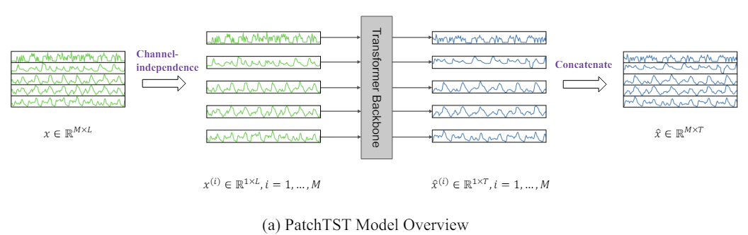
Moreover, a multivariate time series is a multi-channel signal, and each input token can represent data from either one channel or multiple channels. Depending on the input token structure, there are different Transformer architecture options. Channel mixing refers to the latter case, where the input token takes a vector of all time series features and projects it into the embedding space to mix the information. On the other hand, channel independence means that each input token contains information from only one channel. This has previously been shown to work well in convolutional and linear models. PatchTST demonstrates the effectiveness of the independent channels approach in Transformer-based models.
The authors of PatchTST highlight the following advantages of the proposed method:
- Reduction on complexity: Patching allows the reduction on time and space complexity of a model, thus increasing its efficiency on larger datasets.
- Improved learning from longer look-back window: Patches allow the model to learn over longer time periods, potentially improving the quality of forecasts.
- Representation learning: The proposed model is not only effective in prediction, but also capable of extracting more complex abstract representations of data, which improves its generalization ability.
The studies presented in the author's paper demonstrate the effectiveness of the proposed method and its potential for various applied problems of time series analysis.
1. PatchTST Algorithm
The PatchTST method is developed for analyzing and forecasting multivariate time series, in which each state of the analyzed system is described by a vector of parameters. In this case, the size of the description vector of each time step contains the same number of parameters with an identical data structure. Thus, we can divide the general multivariate time series into several univariate time series according to the number of parameters describing the state of the system.
As with the methods we have considered previously, we first bring the model's input data into a comparable form by normalizing them. This step is very important. We have already discussed many times that using normalized data at the model input significantly increases the stability of its training process. Moreover, although the PatchTST method implies channel-independent analysis of univariate time series, the analysis is performed with a single set of training parameters. Therefore, it is very important that the analyzed data from all channels is in a comparable form.
The next step is patching univariate time series, which allows modeling local patterns and increases the generalization ability of the model. At this step, the authors of the PatchTST method suggest dividing the time series into patches of fixed size with a fixed step. The method works equally well with overlapped and non-overlapped patches. In the first case, the step is smaller than the patch size, and in the second case, both hyperparameters are equal. Both approaches to patching allow the exploration of local semantic information. The choice of a specific method largely depends on the task and the size of the analyzed input window.
Obviously, the number of patches will be less than the length of the time series. The larger the size of the patching step, the greater the difference. Therefore, the maximum difference between the number of patches and the time series length is achieved for non-overlapping patches. In this case, the reduction is implemented in multiples of the step size. This allows longer lengths of input time series to be analyzed with the same or even lower memory and computing resources.
When analyzing a small input window, it is recommended to use overlapping patches, which will allow for a more qualitative study of local semantic dependencies.
We create patches for each individual univariate time series, but with the same patching parameters for all.
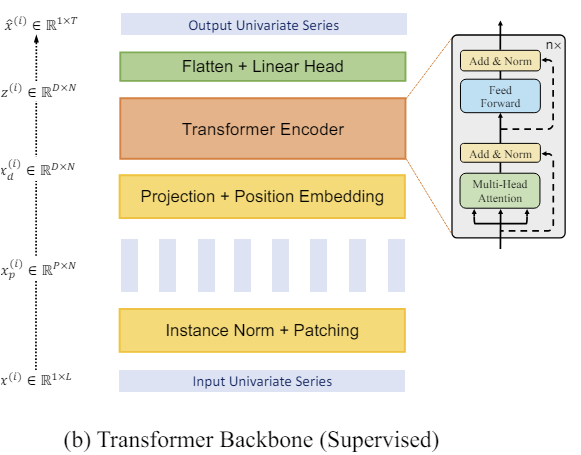
After that we work with the patches that have already been created. We create embeddings for them. We adding trainable positional encoding and pass it to a block of several Vanilla Transformer Encoder layers.
We will not dwell on the Transformer architecture in detail, as we have already discussed it previously. Please note that the Transformer Encoder separately analyzes dependencies within univariate time series. However, the same learning parameters are used to analyze all univariate time series.
Transformer allows extracting abstract representations from input patches, taking into account their time sequence and context. Therefore, the representations obtained at the output of the Encoder contain information about the relationships between patches and the patterns within each of them. The univariate time series representations processed in this way are concatenated. The resulting tensor can be used to solve various problems. It is fed into the "decision head" to generate the model's output.
Please note that the authors of the method propose using one model to solve various problems on one input dataset. This could be searching for anomalies, classification or forecasting subsequent time series data over different planning horizons. You just need to replace the "decision head" and fine-tune (retrain) the model.
When forecasting subsequent time series data. we denormalize the data at the model output by returning statistical characteristics extracted from the input data.
The author's visualization of the method is presented below.
2. Implementing in MQL5
We have considered the theoretical aspects of the method. Now we can move on to the practical implementation of the proposed approaches using MQL5.
Again, we will be implementing our vision of the proposed approaches, which my differ from the original authors' idea.
As follows from the theoretical description of the PatchTST method presented above, it is based on the input patching and the division of the multivariate time series into separate univariate sequences.
The first step in the data processing flow is patching, which is the division of input data into smaller blocks of information. In the case of non-overlapping patches, this can be thought of as reformatting a 2-dimensional input tensor into a 3-dimensional one. For overlapping patches, it is a little more complicated as it requires copying data. But in any case, we get at the output a 3-dimensional tensor: "number of variables * number of patches * patch size".
The transformation of the input data tensor implies data copying operations. We would like to eliminate unnecessary operations, including copying. Because every additional operation is an expense of our time and resources.
Let's pay attention to the following operations. Next in the operations flow is data embedding. A logical solution would be to combine the two operations. Actually, we will only perform the data embedding operation. However, to perform the operation, we will take individual blocks from the input data tensor that correspond to our patches.
We have previously considered convolutional layers. In these layers, we also take an input block in the size of a given window and, after a convolution operation with several filters, we obtain a projection vector of the analyzed data window into a certain subspace. Looks like what we need. But the convolutional layer we created earlier works with a one-dimensional input tensor. It does not allow us to isolate individual univariate time series from the general tensor of a multivariate time series. So we have to create something similar, but with the ability to work within individual univariate sequences.
2.1 OpenCL-side patching
First, let's supplement the OpenCL program, creating kernels for the feed-forward and backward data patching passes, with their projection into a certain subspace of embeddings. Let's start with the feed-forward pass kernel PatchCreate.
In the kernel parameters, we pass pointers to 3 data buffers: inputs, weights matrix and outputs. In addition, we will add 4 constants to the kernel parameters. In these constants, we will specify the full size of the input data tensor to prevent an out-of-range error. We specify the patch size and step. We will also provide the user with the ability to add an activation function.
__kernel void PatchCreate(__global float *inputs,
                          __global float *weights,
                          __global float *outputs,
                          int inputs_total,
                          int window_in,
                          int step,
                          int activation
                         )
  {
   const int i = get_global_id(0);
   const int w = get_global_id(1);
   const int v = get_global_id(2);
   const int window_out = get_global_size(1);
   const int variables = get_global_size(2);
We expect that the kernel will be executed in a 3-dimensional task space: the number of patches, the position of the element in the embedding vector of the analyzed patch, and the identifier of the variable in the source data. Let me remind you that we are constructing segmentation within the framework of independent univariate time series.
In the kernel body we identify the thread across all 3 dimensions of the task space. We also determine the dimensions of the task space.
Then, based on the received data, we can determine the shift in the data buffers to the analyzed elements.
   const int shift_in = i * step * variables + v;
   const int shift_out = (i * variables + v) * window_out + w;
   const int shift_weights = (window_in + 1) * (v * window_out + w);
When determining the shift in the input buffer, we make the following assumptions:
- The input tensor contains a sequence of vectors describing the state of the environment at a separate time step. In other words, the input tensor is a 2-dimensional matrix in which rows contain descriptions of the state of the environment at a particular time step. The columns of the matrix correspond to individual parameters (variables) describing the state of the analyzed environment.
- The PatchTST method analyzes individual univariate time series. Therefore, each parameter (variable) describing the state of the environment contains only 1 element in the vector and is patched independently from the others (within the entire time series).
Remember these assumptions. In accordance with them, we need to prepare the input data on the side of the main program before transferring it to the model.
Next, we organize a loop to multiply the segment vector by the corresponding weights vector. In the loop body, we control the shift in the input data buffer to prevent accesses outside the array bounds.
   float res = weights[shift_weights + window_in];
   for(int p = 0; p < window_in; p++)
      if((shift_in + p * variables) < inputs_total)
         res += inputs[shift_in + p * variables] * weights[shift_weights + p];
   if(isnan(res))
      res = 0;
Note here that when accessing the input tensor data, we use a step equal to the number of variables in the description of one state of the environment. That is, we move along the column of the input matrix. This meets the patching requirement of a univariate time series.
If we receive NaN as a result of the vector multiplication operation, we replace it with "0".
Next, we just need to execute the given activation function and save the resulting value in the corresponding result buffer.
   switch(activation)
     {
      case 0:
         res = tanh(res);
         break;
      case 1:
         res = 1 / (1 + exp(-clamp(res, -20.0f, 20.0f)));
         break;
      case 2:
         if(res < 0)
            res *= 0.01f;
         break;
      defaultд:
         break;
     }
//---
   outputs[shift_out] = res;
  }
After implementing the feed-forward pass, we move on to constructing the backpropagation kernels. First, we will create a kernel to propagate the error gradient to the previous layer - PatchHiddenGradient. In the parameters of this kernel, we will pass 4 pointers to data buffers:
- inputs — input data buffer (necessary for adjusting the error gradients by the derivative of the activation function);
- inputs_gr — buffer of error gradients at the input data level (in this case, a buffer for writing results);
- weights — matrix of trainable parameters of the layer;
- outputs_gr — tensor of gradients at the layer output level (in this case, the input data for calculating the error gradients).
In addition, we will pass 5 constants to the kernel. Their purpose can be easily guessed from the names of the variables.
__kernel void PatchHiddenGradient(__global float *inputs,
                                  __global float *inputs_gr,
                                  __global float *weights,
                                  __global float *outputs_gr,
                                  int window_in,
                                  int step,
                                  int window_out,
                                  int outputs_total,
                                  int activation
                                 )
  {
   const int i = get_global_id(0);
   const int v = get_global_id(1);
   const int variables = get_global_size(1);
We are planning to use the kernel in a 2-dimensional task space: the length of the input sequence and the number of analyzed parameters of the state of the environment (variables).
Note that when constructing kernels, we orient the task space in the dimensions of the output tensor. In the feed-forward pass, we oriented on the 3-dimensional tensor of data embeddings. During the backpropagation pass, it is the 2-dimensional tensor of inputs, or rather their error gradients. This approach allows each individual thread to be configured to receive a single value in the kernel's output buffer.
In the kernel body, we identify the thread in the task space and define the required dimensions. After that we calculate the shifts.
   const int w_start = i % step;
   const int r_start = max((i - window_in + step) / step, 0);
   int total = (window_in - w_start + step - 1) / step;
   total = min((i + step) / step, total);
Then we organize a system of nested loops to collect error gradients.
   float grad = 0;
   for(int p = 0; p < total; p ++)
     {
      int row = r_start + p;
      if(row >= outputs_total)
         break;
      for(int wo = 0; wo < window_out; wo++)
        {
         int shift_g = (row * variables + v) * window_out + wo;
         int shift_w = v * (window_in + 1) * window_out + w_start + (total - p - 1) * step + wo * (window_in + 1);
         grad += outputs_gr[shift_g] * weights[shift_w];
        }
     }
One input element influences the value of all elements of the embedding vector of a single patch with different weights. Therefore, the nested loop collects error gradients from the entire embedding vector of a single patch.
In addition, in the case of overlapping patches, there is a possibility that the analyzed input element data will fall into the input window of several patches. The outer loop of our nested loop system is used to collect the error gradient from such patches.
We adjust the collected (total) error gradient for the analyzed input element by the derivative of the activation function.
   float inp = inputs[i * variables + v];
   if(isnan(grad))
      grad = 0;
//---
   switch(activation)
     {
      case 0:
         grad = clamp(grad + inp, -1.0f, 1.0f) - inp;
         grad = grad * (1 - pow(inp == 1 || inp == -1 ? 0.99999999f : inp, 2));
         break;
      case 1:
         grad = clamp(grad + inp, 0.0f, 1.0f) - inp;
         grad = grad * (inp == 0 || inp == 1 ? 0.00000001f : (inp * (1 - inp)));
         break;
      case 2:
         if(inp < 0)
            grad *= 0.01f;
         break;
      default:
         break;
     }
We write the result of the operations into the corresponding element of the error gradient buffer of the previous neural layer.
   inputs_gr[i * variables + v] = grad;
  }
After propagating the error gradient, we need to adjust the model's training parameters in order to minimize the error. To implement this functionality, we will create the PatchUpdateWeightsAdam kernel, in which we will optimize parameters using the Adam method.
In the kernel parameters, we will pass pointers to 5 data buffers. In addition to the familiar buffers inputs, weights and output_gr, we have auxiliary buffers of the 1st and 2nd moments of the error gradients at the weight matrix level weights_m and weights_v, respectively. In addition, we will also pass learning rates in the kernel parameters.
__kernel void PatchUpdateWeightsAdam(__global float *weights,
                                     __global const float *outputs_gr,
                                     __global const float *inputs,
                                     __global float *weights_m,
                                     __global float *weights_v,
                                     const int inputs_total,
                                     const float l,
                                     const float b1,
                                     const float b2,
                                     int step
                                    )
  {
   const int c = get_global_id(0);
   const int r = get_global_id(1);
   const int v = get_global_id(2);
   const int window_in = get_global_size(0) - 1;
   const int window_out = get_global_size(1);
   const int variables = get_global_size(2);
Since our tensor of weights is 3-dimensional, the task space will also be formed in 3 dimensions:
- patch size + bias,
- embedding vector size,
- number of variables.
Here we follow the logic mentioned above, where each individual thread adjusts the value of 1 trainable parameter.
In the kernel body, we identify the thread in all 3 dimensions of the task space. We also determine the sizes of the dimensions. After that we define shift constants in data buffers.
   const int start_input = c * variables + v;
   const int step_input = step * variables;
   const int start_out = v * window_out + r;
   const int step_out = variables * window_out;
   const int total = inputs_total / (variables * step);
Run a loop to collect error gradients at the level of the corrected learning parameter.
   float grad = 0;
   for(int p = 0; p < total; p++)
     {
      int i = start_input + i * step_input;
      int o = start_out + i * step_out;
      grad += (c == window_in ? 1 : inputs[i]) * outputs_gr[0];
     }
   if(isnan(grad))
      grad = 0;
After determining the error gradient, we move on to the parameter correction algorithm. First, we define the 1st and 2nd order moments.
   const int shift_weights = (window_in + 1) * (window_out * v + r) + c;
//---
   float weight = weights[shift_weights];
   float mt = b1 * weights_m[shift_weights] + (1 - b1) * grad;
   float vt = b2 * weights_v[shift_weights] + (1 - b2) * pow(grad, 2);
Then we calculate the parameter adjustment value.
float delta = l * (mt / (sqrt(vt) + 1.0e-37f) - (l1 * sign(weight) + l2 * weight));
And finally, we will adjust the values in the data buffers.
   if(fabs(delta) > 0)
      weights[shift_weights] = clamp(weight + delta, -MAX_WEIGHT, MAX_WEIGHT);
   weights_m[shift_weights] = mt;
   weights_v[shift_weights] = vt;
  }
Please note that we change the weight in the data buffer only if the parameter change value is different from "0". From a mathematical point of view, adding "0" to the current value does not change the parameter. But we introduce an additional local variable check operation to eliminate the unnecessary, more expensive operation of accessing the global data buffer.
This concludes our work on the OpenCL side. Let's move on to the main program side.
2.2 Data patching class
To call and service the above created kernels on the main program side, we create the CNeuronPatching class, which is inherited from our base class of all neural layers CNeuronBaseOCL.
In the class body, we will declare variables to store the main parameters of the object's architecture, as well as buffers of training parameters and corresponding moments. We declare all buffers as static objects, which allows us to leave the class constructor and destructor "empty".
class CNeuronPatching   :  public CNeuronBaseOCL
  {
protected:
   uint              iWindowIn;
   uint              iStep;
   uint              iWindowOut;
   uint              iVariables;
   uint              iCount;
   //---
   CBufferFloat      cPatchWeights;
   CBufferFloat      cPatchFirstMomentum;
   CBufferFloat      cPatchSecondMomentum;
   //---
   virtual bool      feedForward(CNeuronBaseOCL *NeuronOCL);
   virtual bool      updateInputWeights(CNeuronBaseOCL *NeuronOCL);
   virtual bool      calcInputGradients(CNeuronBaseOCL *NeuronOCL);

public:
                     CNeuronPatching(void){};
                    ~CNeuronPatching(void){};
   //---
   virtual bool      Init(uint numOutputs, uint myIndex, COpenCLMy *open_cl, uint window_in,
                          uint step, uint window_out, uint count, uint variables,
                          ENUM_OPTIMIZATION optimization_type, uint batch);
   //---
   virtual bool      Save(int const file_handle);
   virtual bool      Load(int const file_handle);
   //---
   virtual int       Type(void)        const                      {  return defNeuronPatchingOCL; }
   virtual void      SetOpenCL(COpenCLMy *obj);
   //---
   virtual bool      WeightsUpdate(CNeuronBaseOCL *source, float tau);
  };
The set of overridable class methods is quite standard. Objects and class variables are initialized in the Init method. In the parameters, the method receives all the necessary information to create an object of the required architecture.
bool CNeuronPatching::Init(uint numOutputs, uint myIndex, COpenCLMy *open_cl,
                           uint window_in, uint step, uint window_out,
                           uint count, uint variables,
                           ENUM_OPTIMIZATION optimization_type, uint batch
                          )
  {
   if(!CNeuronBaseOCL::Init(numOutputs, myIndex, open_cl, window_out * count * variables,
                                                                optimization_type, batch))
      return false;
In the body of the method, we first call the same method of the parent class, which performs the minimum necessary control of the received values and initialization of inherited objects and variables. The result of executing operations in the parent class method is controlled by the returned logical value.
After successful execution of operations in the parent class method, we save the obtained values of the object architecture description in local variables.
   iWindowIn = MathMax(window_in, 1);
   iWindowOut = MathMax(window_out, 1);
   iStep = MathMax(step, 1);
   iVariables = MathMax(variables, 1);
   iCount = MathMax(count, 1);
Initialize the buffer of training parameters.
   int total = int((window_in + 1) * window_out * variables);
   if(!cPatchWeights.Reserve(total))
      return false;
   float k = float(1 / sqrt(total));
   for(int i = 0; i < total; i++)
     {
      if(!cPatchWeights.Add((2 * GenerateWeight()*k - k)*WeightsMultiplier))
         return false;
     }
   if(!cPatchWeights.BufferCreate(OpenCL))
      return false;
Also initialize buffers of moments of the error gradient at the level of the training parameters.
   if(!cPatchFirstMomentum.BufferInit(total, 0) ||
      !cPatchFirstMomentum.BufferCreate(OpenCL))
      return false;
   if(!cPatchSecondMomentum.BufferInit(total, 0) ||
      !cPatchSecondMomentum.BufferCreate(OpenCL))
      return false;
//---
   return true;
  }
After initializing the object, we move on to constructing the feed-forward method CNeuronPatching::feedForward. In this method we enqueue the above created feed-forward pass kernel. We have already described the procedures for placing a kernel in the execution queue several times in previous articles. The main attention here should be paid to the correct indication of size for the task space and the parameters we are passing.
As we already mentioned when constructing the kernel, in this case we use a 3-dimensional task space:
- number of patches
- 1 patch embedding size
- number of parameters analyzed in the description of the state of the environment
bool CNeuronPatching::feedForward(CNeuronBaseOCL *NeuronOCL)
  {
   if(!NeuronOCL || !OpenCL)
      return false;
//---
   uint global_work_offset[3] = {0, 0, 0};
   uint global_work_size[3] = {iCount, iWindowOut, iVariables};
After creating the task space indication arrays and the shifts in it, we organize the process of passing parameters to the kernel.
   ResetLastError();
   if(!OpenCL.SetArgumentBuffer(def_k_PatchCreate, def_k_ptc_inputs, NeuronOCL.getOutputIndex()))
     {
      printf("Error of set parameter kernel %s: %d; line %d", __FUNCTION__, GetLastError(), __LINE__);
      return false;
     }
   if(!OpenCL.SetArgumentBuffer(def_k_PatchCreate, def_k_ptc_weights, cPatchWeights.GetIndex()))
     {
      printf("Error of set parameter kernel %s: %d; line %d", __FUNCTION__, GetLastError(), __LINE__);
      return false;
     }
   if(!OpenCL.SetArgumentBuffer(def_k_PatchCreate, def_k_ptc_outputs, Output.GetIndex()))
     {
      printf("Error of set parameter kernel %s: %d; line %d", __FUNCTION__, GetLastError(), __LINE__);
      return false;
     }
   if(!OpenCL.SetArgument(def_k_PatchCreate, def_k_ptc_activation, (int)activation))
     {
      printf("Error of set parameter kernel %s: %d; line %d", __FUNCTION__, GetLastError(), __LINE__);
      return false;
     }
   if(!OpenCL.SetArgument(def_k_PatchCreate, def_k_ptc_inputs_total, (int)NeuronOCL.Neurons()))
     {
      printf("Error of set parameter kernel %s: %d; line %d", __FUNCTION__, GetLastError(), __LINE__);
      return false;
     }
   if(!OpenCL.SetArgument(def_k_PatchCreate, def_k_ptc_window_in, (int)iWindowIn))
     {
      printf("Error of set parameter kernel %s: %d; line %d", __FUNCTION__, GetLastError(), __LINE__);
      return false;
     }
   if(!OpenCL.SetArgument(def_k_PatchCreate, def_k_ptc_step, (int)iStep))
     {
      printf("Error of set parameter kernel %s: %d; line %d", __FUNCTION__, GetLastError(), __LINE__);
      return false;
     }
Do not forget to control the correctness of the operations. After successfully transferring all the necessary parameters, we place the kernel in the execution queue.
   if(!OpenCL.Execute(def_k_PatchCreate, 3, global_work_offset, global_work_size))
     {
      printf("Error of execution kernel %s: %d", __FUNCTION__, GetLastError());
      return false;
     }
//---
   return true;
  }
Similarly, we place the error gradient distribution kernel in the queue before the elements of the previous layer in accordance with their influence on the final result of the model in the CNeuronPatching::calcInputGradients method. The PatchHiddenGradient kernel is called in a 2-dimensional task space.
bool CNeuronPatching::calcInputGradients(CNeuronBaseOCL *NeuronOCL)
  {
   if(!NeuronOCL || !OpenCL)
      return false;
//---
   uint global_work_offset[2] = {0, 0};
   uint global_work_size[2] = {NeuronOCL.Neurons() / iVariables, iVariables};
It should be noted here that we define the size of the input sequence of a multivariate time series as the ratio of the size of the previous layer results buffer to the number of analyzed variables describing 1 the state of the environment.
Let me remind you that according to the PatchTST method, the input should be a multivariate time series, in which each state of the environment is described by a vector of fixed length. Each element of the vector contains the value of the corresponding parameter describing the state of the system.
Next, we pass the parameters to the kernel and control the execution of operations.
   ResetLastError();
   if(!OpenCL.SetArgumentBuffer(def_k_PatchHiddenGradient, def_k_pthg_inputs, NeuronOCL.getOutputIndex()))
     {
      printf("Error of set parameter kernel %s: %d; line %d", __FUNCTION__, GetLastError(), __LINE__);
      return false;
     }
   if(!OpenCL.SetArgumentBuffer(def_k_PatchHiddenGradient, def_k_pthg_inputs_gr, NeuronOCL.getGradientIndex()))
     {
      printf("Error of set parameter kernel %s: %d; line %d", __FUNCTION__, GetLastError(), __LINE__);
      return false;
     }
   if(!OpenCL.SetArgumentBuffer(def_k_PatchHiddenGradient, def_k_pthg_weights, cPatchWeights.GetIndex()))
     {
      printf("Error of set parameter kernel %s: %d; line %d", __FUNCTION__, GetLastError(), __LINE__);
      return false;
     }
   if(!OpenCL.SetArgumentBuffer(def_k_PatchHiddenGradient, def_k_pthg_outputs_gr, Gradient.GetIndex()))
     {
      printf("Error of set parameter kernel %s: %d; line %d", __FUNCTION__, GetLastError(), __LINE__);
      return false;
     }
   if(!OpenCL.SetArgument(def_k_PatchHiddenGradient, def_k_pthg_activation, (int)NeuronOCL.Activation()))
     {
      printf("Error of set parameter kernel %s: %d; line %d", __FUNCTION__, GetLastError(), __LINE__);
      return false;
     }
   if(!OpenCL.SetArgument(def_k_PatchHiddenGradient, def_k_pthg_outputs_total, (int)iCount))
     {
      printf("Error of set parameter kernel %s: %d; line %d", __FUNCTION__, GetLastError(), __LINE__);
      return false;
     }
   if(!OpenCL.SetArgument(def_k_PatchHiddenGradient, def_k_pthg_window_in, (int)iWindowIn))
     {
      printf("Error of set parameter kernel %s: %d; line %d", __FUNCTION__, GetLastError(), __LINE__);
      return false;
     }
   if(!OpenCL.SetArgument(def_k_PatchHiddenGradient, def_k_pthg_step, (int)iStep))
     {
      printf("Error of set parameter kernel %s: %d; line %d", __FUNCTION__, GetLastError(), __LINE__);
      return false;
     }
   if(!OpenCL.SetArgument(def_k_PatchHiddenGradient, def_k_pthg_window_out, (int)iWindowOut))
     {
      printf("Error of set parameter kernel %s: %d; line %d", __FUNCTION__, GetLastError(), __LINE__);
      return false;
     }
Put the kernel into the execution queue.
   if(!OpenCL.Execute(def_k_PatchHiddenGradient, 2, global_work_offset, global_work_size))
     {
      printf("Error of execution kernel %s: %d", __FUNCTION__, GetLastError());
      return false;
     }
//---
   return true;
  }
The last method to consider in this class is the method that adjusts the model's trainable parameters CNeuronPatching::updateInputWeights. This method is used to place the PatchUpdateWeightsAdam kernel to a queue. Its algorithm is described above. The algorithm for placing the kernel in the execution queue is identical to the two methods described above. However, the difference is in the details. A 3-dimensional task space is used here.
bool CNeuronPatching::updateInputWeights(CNeuronBaseOCL *NeuronOCL)
  {
   if(!NeuronOCL || !OpenCL)
      return false;
//---
   uint global_work_offset[3] = {0, 0, 0};
   uint global_work_size[3] = {iWindowIn + 1, iWindowOut, iVariables};
In the first dimension, we add 1 element of Bayesian bias to the patch size. In the second and third dimensions, we specify the embedding size of 1 patch and the number of analyzed independent channels stored in our class variables.
Then we transfer parameters to the kernel and control the results of the operations.
   ResetLastError();
   if(!OpenCL.SetArgumentBuffer(def_k_PatchUpdateWeightsAdam, def_k_ptuwa_inputs, NeuronOCL.getOutputIndex()))
     {
      printf("Error of set parameter kernel %s: %d; line %d", __FUNCTION__, GetLastError(), __LINE__);
      return false;
     }
   if(!OpenCL.SetArgumentBuffer(def_k_PatchUpdateWeightsAdam, def_k_ptuwa_outputs_gr, getGradientIndex()))
     {
      printf("Error of set parameter kernel %s: %d; line %d", __FUNCTION__, GetLastError(), __LINE__);
      return false;
     }
   if(!OpenCL.SetArgumentBuffer(def_k_PatchUpdateWeightsAdam, def_k_ptuwa_weights, cPatchWeights.GetIndex()))
     {
      printf("Error of set parameter kernel %s: %d; line %d", __FUNCTION__, GetLastError(), __LINE__);
      return false;
     }
   if(!OpenCL.SetArgumentBuffer(def_k_PatchUpdateWeightsAdam, def_k_ptuwa_weights_m,
                                                                            cPatchFirstMomentum.GetIndex()))
     {
      printf("Error of set parameter kernel %s: %d; line %d", __FUNCTION__, GetLastError(), __LINE__);
      return false;
     }
   if(!OpenCL.SetArgumentBuffer(def_k_PatchUpdateWeightsAdam, def_k_ptuwa_weights_v,
                                                                           cPatchSecondMomentum.GetIndex()))
     {
      printf("Error of set parameter kernel %s: %d; line %d", __FUNCTION__, GetLastError(), __LINE__);
      return false;
     }
   if(!OpenCL.SetArgument(def_k_PatchUpdateWeightsAdam, def_k_ptuwa_inputs_total, (int)NeuronOCL.Neurons()))
     {
      printf("Error of set parameter kernel %s: %d; line %d", __FUNCTION__, GetLastError(), __LINE__);
      return false;
     }
   if(!OpenCL.SetArgument(def_k_PatchUpdateWeightsAdam, def_k_ptuwa_l, lr))
     {
      printf("Error of set parameter kernel %s: %d; line %d", __FUNCTION__, GetLastError(), __LINE__);
      return false;
     }
   if(!OpenCL.SetArgument(def_k_PatchUpdateWeightsAdam, def_k_ptuwa_b1, b1))
     {
      printf("Error of set parameter kernel %s: %d; line %d", __FUNCTION__, GetLastError(), __LINE__);
      return false;
     }
   if(!OpenCL.SetArgument(def_k_PatchUpdateWeightsAdam, def_k_ptuwa_step, (int)iStep))
     {
      printf("Error of set parameter kernel %s: %d; line %d", __FUNCTION__, GetLastError(), __LINE__);
      return false;
     }
   if(!OpenCL.SetArgument(def_k_PatchUpdateWeightsAdam, def_k_ptuwa_b2, b2))
     {
      printf("Error of set parameter kernel %s: %d; line %d", __FUNCTION__, GetLastError(), __LINE__);
      return false;
     }
After that, the kernel is placed in the execution queue.
   if(!OpenCL.Execute(def_k_PatchUpdateWeightsAdam, 3, global_work_offset, global_work_size))
     {
      printf("Error of execution kernel %s: %d", __FUNCTION__, GetLastError());
      return false;
     }
//---
   return true;
  }
The class also has file operation methods, which you can study using the codes attached below. In addition to file operations, attachments include all classes and methods for creating and training models.
We have created a method for generating patch embeddings, which are created for independent univariate time series that are constituent parts of the analyzed multivariate time series. However, this is only half of the proposed PatchTST method. The second important block of this method is Transformer for analyzing dependencies between patches within a univariate time series. Please note that the analysis of dependencies is performed only within the framework of independent channels. There is no analysis of cross-dependencies between elements of different univariate channels.
All the Transformer architecture implementation options we have considered earlier used channel mixing, which contradicts the principles of the PatchTST method. The only exception is Conformer. Although, Conformer, unlike vanilla Transformer used by the authors of the PatchTST method, has a more complex architecture. It uses Continuous Attention and NeuralODE blocks to improve the efficiency of the model, which generally gives a positive result. This was confirmed by our experiments. Therefore, as part of my implementation, I boldly replaced Transformer used by the PatchTST authors with the implementation of the previously created Conformer block in class CNeuronConformer.
2.3 Model architecture
After implementing the "blocks" for the PatchTST method, we move on to creating the architecture of trainable models. The method under consideration was proposed for forecasting multivariate time series. Obviously, we'll implement this method within the Environment State Encoder. The architecture of this model is described in the CreateEncoderDescriptions method. In its parameters, we only pass one pointer to a dynamic array to preserve the model architecture.
bool CreateEncoderDescriptions(CArrayObj *encoder)
  {
//---
   CLayerDescription *descr;
//---
   if(!encoder)
     {
      encoder = new CArrayObj();
      if(!encoder)
         return false;
     }
In the method body, we check the relevance of the received pointer to the object and, if necessary, create a new instance of the dynamic array.
We feed the model with a complete set of historical data.
//--- Encoder
   encoder.Clear();
//--- Input layer
   if(!(descr = new CLayerDescription()))
      return false;
   descr.type = defNeuronBaseOCL;
   int prev_count = descr.count = (HistoryBars * BarDescr);
   descr.activation = None;
   descr.optimization = ADAM;
   if(!encoder.Add(descr))
     {
      delete descr;
      return false;
     }
It is worth noting here that the patch creation procedure does not allow using a history depth of less than 1 input patch. Of course, we can only feed historical data of 1 patch depth at each call. Then, the entire depth of the analyzed history would be accumulated in the internal stack, as we did earlier in the Embedding layer. But this approach has a number of limitations. First of all, we would need to specify a step between patches equal to the patch itself (non-overlapping patches). But the actual step would be equal to the model call frequency.
So, there would be some confusion and complexity here in aligning the programs for collecting training data, training and operating models.
The second point is that with this approach, when changing the patch size or step, we would need to re-collect the training sample. This would introduce additional restrictions and costs into the process of training models.
Therefore, we use a simpler and more universal method of feeding the model the full depth of the analyzed history. The patch and step size are set by parameters in the architecture of the corresponding model layer.
As always, we feed the model with "raw" unprocessed data, which we immediately normalize in the batch normalization layer.
//--- layer 1
   if(!(descr = new CLayerDescription()))
      return false;
   descr.type = defNeuronBatchNormOCL;
   descr.count = prev_count;
   descr.batch = 1000;
   descr.activation = None;
   descr.optimization = ADAM;
   if(!encoder.Add(descr))
     {
      delete descr;
      return false;
     }
Next, it should be noted that in this model, the layer of trainable positional encoding is placed at the input level, not at embeddings, as was done previously. In this way I wanted to focus on the position of specific parameters. When using overlapping patches, one parameter can be included in several patches.
//--- layer 2
   if(!(descr = new CLayerDescription()))
      return false;
   descr.type = defNeuronLearnabledPE;
   descr.count = prev_count;
   if(!encoder.Add(descr))
     {
      delete descr;
      return false;
     }
Next I added a Dropout layer, which we will use to mask individual input values during the model training process.
//--- layer 3
   if(!(descr = new CLayerDescription()))
      return false;
   descr.type = defNeuronDropoutOCL;
   descr.count = prev_count;
   descr.probability = 0.4f;
   descr.activation = None;
   if(!encoder.Add(descr))
     {
      delete descr;
      return false;
     }
I set the data masking coefficient at 40%, similar to the previous work.
Then we add a patch generation layer. In my work, I used non-overlapping patches with a window size and step size equal to 3.
//--- layer 4
   if(!(descr = new CLayerDescription()))
      return false;
   descr.type = defNeuronPatchingOCL;
   descr.window = 3;
   prev_count = descr.count = (HistoryBars+descr.window-1)/descr.window;
   descr.step = descr.window;
   descr.layers=BarDescr;
   int prev_wout = descr.window_out = EmbeddingSize / 2;
   if(!encoder.Add(descr))
     {
      delete descr;
      return false;
     }
Here it is also worth noting that the patch embedding is formed in 2 stages. First, we generate patch embeddings at half the size. Then, in the convolution layer, we increase the patch size.
//--- layer 5
   if(!(descr = new CLayerDescription()))
      return false;
   descr.type = defNeuronConvOCL;
   descr.count = prev_count*BarDescr;
   descr.window = prev_wout;
   descr.step = prev_wout;
   prev_wout = descr.window_out = EmbeddingSize;
   if(!encoder.Add(descr))
     {
      delete descr;
      return false;
     }
As you remember, we implemented positional encoding at the input level. Therefore, after generating the embeddings, we immediately put the data into the 10-layer Conformer block.
//--- layer 6-16
   for(int i = 0; i < 10; i++)
     {
      if(!(descr = new CLayerDescription()))
         return false;
      descr.type = defNeuronConformerOCL;
      descr.count = prev_count;
      descr.window = prev_wout;
      descr.step = 8;
      descr.window_out = EmbeddingSize;
      descr.layers = BarDescr;
      if(!encoder.Add(descr))
        {
         delete descr;
         return false;
        }
     }
Next comes the decision head, which consists of 3 fully connected layers. We make the size of the last layer sufficient to contain the reconstructed information of historical data and to predict subsequent states to a given depth.
//--- layer 17
   if(!(descr = new CLayerDescription()))
      return false;
   descr.type = defNeuronBaseOCL;
   descr.count = LatentCount;
   descr.activation=SIGMOID;
   if(!encoder.Add(descr))
     {
      delete descr;
      return false;
     }
//--- layer 18
   if(!(descr = new CLayerDescription()))
      return false;
   descr.type = defNeuronBaseOCL;
   descr.count = LatentCount;
   descr.activation=LReLU;
   if(!encoder.Add(descr))
     {
      delete descr;
      return false;
     }
//--- layer 19
   if(!(descr = new CLayerDescription()))
      return false;
   descr.type = defNeuronBaseOCL;
   prev_count=descr.count = BarDescr*(HistoryBars+NForecast);
   descr.activation=TANH;
   if(!encoder.Add(descr))
     {
      delete descr;
      return false;
     }
At the end of the model, we denormalize the reconstructed and predicted values by adding statistical indicators extracted from the original data.
//--- layer 20
   if(!(descr = new CLayerDescription()))
      return false;
   descr.type = defNeuronRevInDenormOCL;
   prev_count = descr.count = prev_count;
   descr.activation = None;
   descr.optimization = ADAM;
   descr.layers = 1;
   if(!encoder.Add(descr))
     {
      delete descr;
      return false;
     }
//---
   return true;
  }
Please note that we have left the size of the input data and model results the same as in the previous article. Therefore, we can copy the Actor and Critic models without changes. Moreover, in the new experiment, we can use the training dataset and EAs from the previous articles. In this way, we can compare the impact of different environment state encoder architectures on the Actor policy learning results.
The attachments contain the complete architecture description for all trainable models used herein.
3. Testing
In the previous sections of this article, we introduced a new method for forecasting multivariate time series, PatchTST. We have implemented our vision of the proposed approaches using MQL5. Now it's time to test the work done. We first train the models using real historical data. Then we test the trained models in the MetaTrader 5 strategy tester on a historical period beyond the training dataset.
As before, the model is trained on EURUSD H1 historical data. The trained model is tested using historical data for January, 2024, with the same financial instrument and timeframe. While collecting the training sample and testing the learned policy, we used indicators with default parameters.
The models are trained in two stages. In the first step, we train the environment state encoder. This model learns to analyze and generalize only historical data of multivariate time series of the symbol price dynamics and analyzed indicators. The process does not take into account the account state and open positions. Therefore, we train the model on the initial training dataset without collecting additional data until we obtain an acceptable result in reconstructing the masked data and predicting subsequent states.
At the second stage, we train the Actor's behavior policy and the correctness of the Critic's assessments of actions. This stage is iterative and includes 2 subprocesses:
- Training Actor and Critic models.
- Collection of additional environmental data taking into account the Actor's current policy.
After several Actor training iterations, I obtained a model capable of generating profits both on historical training data and on new data. The results of the trained model on new data are presented below.
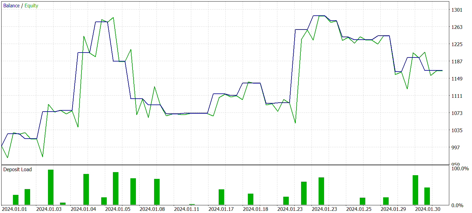
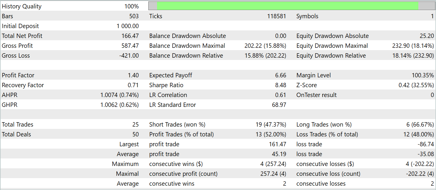
The balance graph cannot be considered as smoothly increasing. Nevertheless, during the testing period, the model made 25 trades, of which 13 were closed with a profit. This amounted to 52.0% of profitable trades. The value is close to parity. However, the maximum winning trade exceeds the maximum losing one by 87.2%, and the average winning trade exceeds the average losing one by 28.6%. As a result, during the testing period, the profit factor was 1.4.
Conclusion
In this article, we have discussed a new method for analyzing and forecasting multidimensional time series, PatchTST, which combines the benefits of data patching, transformer use, and representation learning. Data patching allows the model to better capture local temporal patterns and context, which improves the quality of analysis and prediction. The use of a transformer allows us to extract abstract representations from data, taking into account their time oral sequence and interrelationships.
In the practical part of the article, we implemented our vision of the proposed approaches using MQL5. We trained the model using real historical data. Then we tested the trained Actor policy using new data not included in the training sample. The obtained results show that it is possible to use the PatchTST method to build and train models that can generate profit.
The PatchTST method is a powerful tool for analyzing and forecasting multivariate time series, which can be successfully applied in various practical problems.
- A Time Series is Worth 64 Words: Long-term Forecasting with Transformers
- Other articles from this series
Programs used in the article
| # | Name | Type | Description |
|---|---|---|---|
| 1 | Research.mq5 | EA | Example collection EA |
| 2 | ResearchRealORL.mq5 | EA | EA for collecting examples using the Real-ORL method |
| 3 | Study.mq5 | EA | Model training EA |
| 4 | StudyEncoder.mq5 | EA | Encode training EA |
| 5 | Test.mq5 | EA | Model testing EA |
| 6 | Trajectory.mqh | Class library | System state description structure |
| 7 | NeuroNet.mqh | Class library | A library of classes for creating a neural network |
| 8 | NeuroNet.cl | Code Base | OpenCL program code library |
Translated from Russian by MetaQuotes Ltd.
Original article: https://www.mql5.com/ru/articles/14798
Warning: All rights to these materials are reserved by MetaQuotes Ltd. Copying or reprinting of these materials in whole or in part is prohibited.
This article was written by a user of the site and reflects their personal views. MetaQuotes Ltd is not responsible for the accuracy of the information presented, nor for any consequences resulting from the use of the solutions, strategies or recommendations described.

- Free trading apps
- Over 8,000 signals for copying
- Economic news for exploring financial markets
You agree to website policy and terms of use
I have been following the series for a while now, and it has be insightful.
I have one question however; will the entire series be published as a book at the end?
I have been following the series for a while now, and it has be insightful.
I have one question however; will the entire series be published as a book at the end?
Hi,
Dmitriy Gizlyk, the author of this series, has already written a book on neural networks in trading. You can find it here: https://www.mql5.com/en/neurobook. Feel free to download it in pdf or chm.