
Neural Networks Made Easy (Part 83): The "Conformer" Spatio-Temporal Continuous Attention Transformer Algorithm

Introduction
The unpredictability of financial market behavior can probably be compared to the volatility of the weather. However, humanity has done quite a lot in the field of weather forecasting. So, we can now quite trust the weather forecasts provided by meteorologists. Can we use their developments to forecast the "weather" in financial markets? In this article, we will get acquainted with the complex algorithm of the "Conformer" Spatio-Temporal Continuous Attention Transformer, which was developed for the purposes of weather forecasting and is presented in the paper "Conformer: Embedding Continuous Attention in Vision Transformer for Weather Forecasting". In their work, the authors of the method propose the Continuous Attention algorithm. They combine it with those we discussed in the previous article on Neural ODE.
1. The Conformer Algorithm
Conformer is designed to study continuous weather change over time by implementing continuity in the multi-head attention mechanism. The attention mechanism is encoded as a differentiable function in the transformer architecture to model complex weather dynamics.
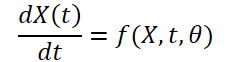
Initially, the authors of the method were faced with the task of building a model that receives weather data as input in the form (XN*W*H, T). Here N is the number of weather variables such as temperature, wind speed, pressure, etc. W*H refers to the spatial resolution of the variable. T is the time during which the system develops. The model receives weather variables over time t, studies the evolution of the spatio-temporal system and predicts the weather at the next time step t+1.
![]()
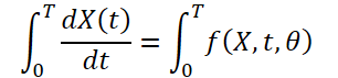
Since the weather is constantly changing over time, it is also important to record the continuous changes within the provided data for a fixed time. The idea is to learn the continuous latent representation of weather data using differential equation solvers. Thus, the model not only predicts the value of the weather variable at time 'T', but the definite integral also studies the changes in the weather variable, such as temperature, from the initial time to time 'T'. The system can be represented as:
![]()
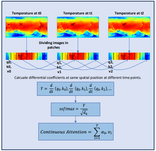
Weather information is highly variable and difficult to predict both temporally and spatially. Time derivatives of each weather variable are calculated to preserve weather dynamics and provide better feature extraction from discrete data. The authors of the method perform selective differentiation at the pixel level to capture continuous changes in weather phenomena over time.
Normalization of derivatives is one of the most important steps to ensure the behavior stability for a deep learning model. The authors of the method expand the idea of normalization as separate elements of the model architecture. They explore the role of normalization when applied directly to derivatives. In this paper, they consider the impact of two most common normalization methods and a pre-differentiation layer on the model's performance to demonstrate their advantages in continuous systems.
Attention is one of the key components of the Transformer architecture. It is based on the idea of identifying the most important blocks of source data at the final forecasting step. Despite its success in solving various problems, Transformer remains limited in its ability to learn information embedding for highly dynamic systems such as weather forecasting. Authors of the Conformer method develop the Continuous Attention mechanism to model continuous changes in the weather variables. First, they replace the analysis of dependencies between elements of the initial state with attention between the corresponding parameters of different states of the environment. This allows the computation of the contextual embedding space for each time-varying weather variable. This step ensures that the model will process the same variable in different states in a batch instead of accessing blocks in the same environment state. Variable transformation is learned by assigning each variable its own Query, Key, and Value for each source data sample, similar to how it is done in a single environment state. The attention mechanism computes dependency estimates between variables in different samples (at the same variable positions). Similar to traditional attention mechanisms, the dependency weights learned for different batches can be used to aggregate or weight the information associated with those variables.
This modification allows the model to capture relationships or dependencies between the same weather variables in different environmental states. This has proven useful in the weather forecasting scenario where the model is able to represent the continuously evolving characteristics of each weather variable. To ensure continuous learning, the authors of the method introduce derivatives into the Continuous Attention mechanism. Differential equations represent the dynamics of a physical system over time and account for missing data values. The authors of the method combined the attention mechanism with the differential equation learning paradigm to model atmospheric changes in both spatial and temporal characteristics. Moreover, this approach removes the limitation related to the modeling of complex physical equations in models. Instead of making forecasts predictions only for a certain time stamp, Conformer learns the transitional changes from one time step to another, which is important for capturing unprecedented changes in the weather.
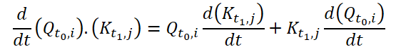
To compute Continuous Attention, the authors of the method propose to compute the derivatives of similarity for the same variables in each data sample. Suppose we have 2 input samples of size (N*W*H). Let's denote them as X0 and X1 at time t0 and t1, respectively. Each variable has its own tensors Q, K and V in both samples. Continuous Attention is computed as follows:
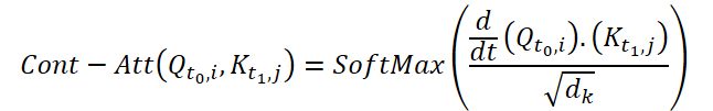
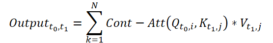
The result obtained is an attention-weighted sum of the values of similar variables in the input data at a certain point in time t0 and t1. The presented process computes attention between similar variables in the input data across all time steps, allowing the model to capture relationships or interactions between variables across the entire sequence of input samples.
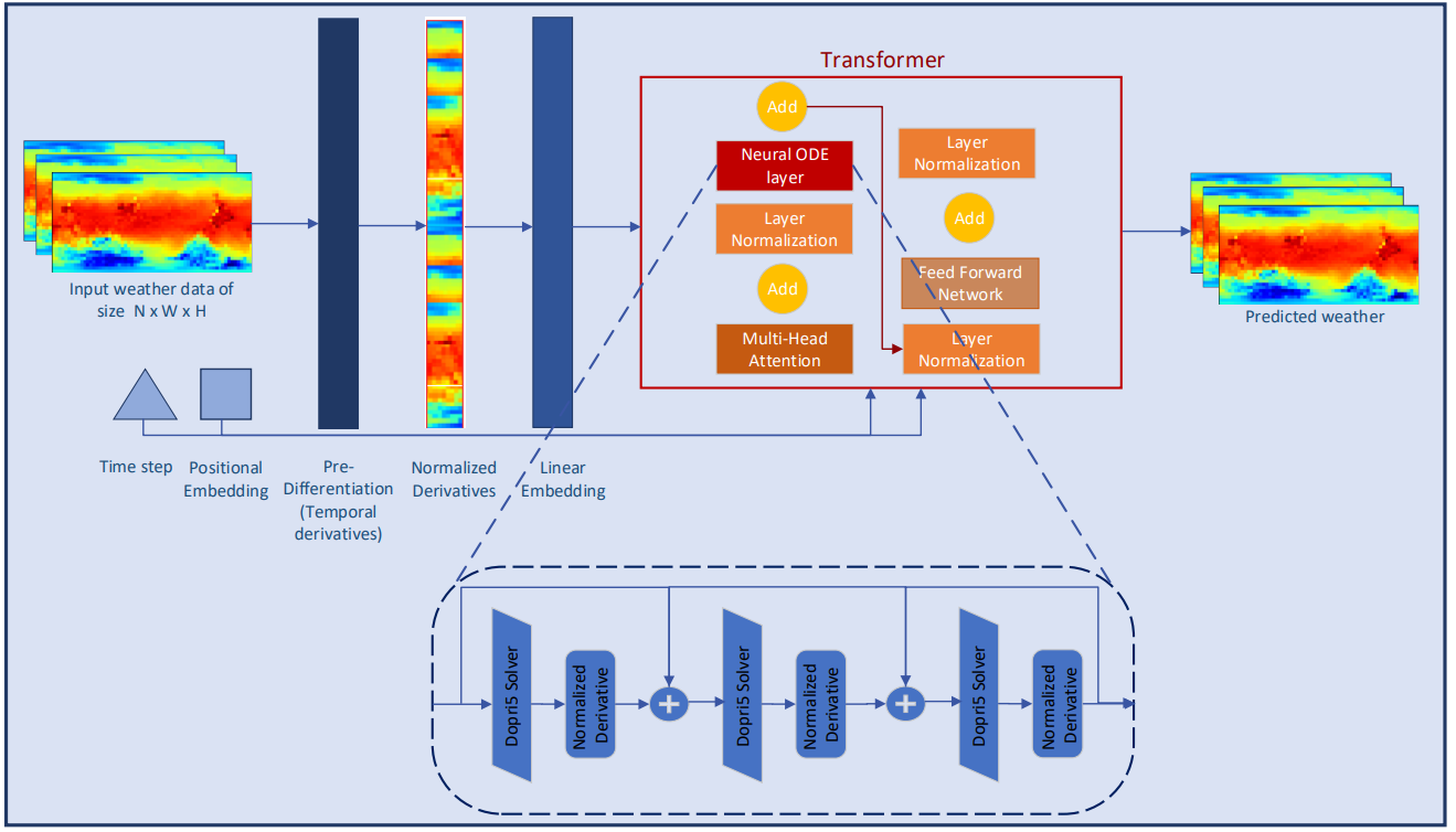
To further explore the continuous characteristics of meteorological information, the authors of Conformer add layers to the Neural ODE model. Since adaptive-size solvers have higher accuracy than fixed-size solvers, the authors of the method chose the Dormand-Prince method (Dopri5). This allows studying the smallest possible changes in weather over time. The complete workflow of Conformer and placement of Neural ODE layers is shown in the author's visualization of the method below.
2. Implementing in MQL5
After reviewing the theoretical aspects of the Conformer methods, we now move on to the practical implementation of the proposed approaches using MQL5. We will implement the main functionality in a new class CNeuronConformer, deriving it from the neural layer base class CNeuronBaseOCL.
2.1 CNeuronConformer class architecture
In the CNeuronConformer class structure, we are already seeing familiar methods that are redefined in all classes implementing attention methods. However Continuous Attention differs so much from the previously considered attention methods. Therefore, I decided to implement the algorithm from scratch. Nevertheless, this implementation will use the developments from previous works.
To write the main parameters of the layer architecture, we introduce 5 variables:
- iWindow – the size of the vector describing one parameter in the initial data tensor.
- iDimension – the dimension of the vector of one Query, Key, Value entity.
- iHeads – number of attention heads.
- iVariables – the number of parameters describing one state of the environment.
- iCount – the number of analyzed states of the environment (length of the sequence of initial data).
To generate Query, Key and Value entities, we, as before in similar cases, use a convolutional layer cQKV. This approach allows us to implement all 3 entities in parallel. We will write the derivatives of entities over time in the base neural layer cdQKV.
The dependency coefficients, similar to the native Transformer algorithm, will be saved in the Score matrix. But in this implementation, we will not create a copy of the matrix on the main program side. We will only create a buffer in the OpenCL context. In the local variable iScore of the CNeuronConformer class we will save the pointer to the buffer.
The results of multi-head attention will be saved in the buffers of the base neural layer AttentionOut. We will reduce the dimensionality of the obtained data using a convolutional layer cW0.
According to the Conformer algorithm, the attention block is followed by a block of neural layers of ordinary differential equations. For them, we will create the cNODE array. Similarly, for the FeedForward block, we will create the cFF array.
class CNeuronConformer  :  public CNeuronBaseOCL
  {
protected:
   //---
   int               iWindow;
   int               iDimension;
   int               iHeads;
   int               iVariables;
   int               iCount;
   //---
   CNeuronConvOCL    cQKV;
   CNeuronBaseOCL    cdQKV;
   int               iScore;
   CNeuronBaseOCL    cAttentionOut;
   CNeuronConvOCL    cW0;
   CNeuronNODEOCL    cNODE[3];
   CNeuronConvOCL    cFF[2];
   //---
   virtual bool      feedForward(CNeuronBaseOCL *NeuronOCL);
   virtual bool      attentionOut(void);
   //---
   virtual bool      AttentionInsideGradients(void);
   virtual bool      updateInputWeights(CNeuronBaseOCL *NeuronOCL);

public:
                     CNeuronConformer(void) {};
                    ~CNeuronConformer(void) {};
   //---
   virtual bool      Init(uint numOutputs, uint myIndex, COpenCLMy *open_cl,
                          uint window, uint window_key, uint heads,
                          uint variables, uint units_count,
                          ENUM_OPTIMIZATION optimization_type,
                          uint batch);
   //---
   virtual bool      calcInputGradients(CNeuronBaseOCL *prevLayer);
   //---
   virtual int       Type(void)   const   {  return defNeuronConformerOCL;   }
   //--- methods for working with files
   virtual bool      Save(int const file_handle);
   virtual bool      Load(int const file_handle);
   //---
   virtual void      SetOpenCL(COpenCLMy *obj);
   virtual CLayerDescription* GetLayerInfo(void);
  };
All internal objects of the class are declared as static. This allows us to leave the class constructor and destructor "empty". The initialization of the class object in accordance with the user requirements is implemented in the Init method. In the method parameters, we pass the main parameters of the object architecture.
bool CNeuronConformer::Init(uint numOutputs, uint myIndex, COpenCLMy *open_cl,
                            uint window, uint window_key, uint heads,
                            uint variables, uint units_count,
                            ENUM_OPTIMIZATION optimization_type, uint batch)
  {
   if(!CNeuronBaseOCL::Init(numOutputs, myIndex, open_cl, window * variables * units_count,
                                                                  optimization_type, batch))
      return false;
In the body of the method, we call the relevant method of the parent class, which implements the minimum necessary control of the received parameters and initialization of inherited objects. We can check the results of the controls and initialization from the logical result returned by the method.
Next, we initialize the inner layer cQKV, which serves to generate the Query, Key and Value entities. Please note that according to the Conformer method, entities are created for each individual variable. Therefore, the window size and convolution step are equal to the length of the embedding vector of one variable. The number of convolution elements is equal to the product of the number of variables describing one state of the environment by the number of such states being analyzed. The number of convolution filters is equal to 3 products of the length of one entity and the number of attention heads.
   if(!cQKV.Init(0, 0, OpenCL, window, window, 3 * window_key * heads, variables * units_count,
                                                                         optimization, iBatch))
      return false;
After successfully completing the 2 methods above, we save the received parameters in internal variables.
   iWindow = int(fmax(window, 1));
   iDimension = int(fmax(window_key, 1));
   iHeads = int(fmax(heads, 1));
   iVariables = int(fmax(variables, 1));
   iCount = int(fmax(units_count, 1));
We initialize the inner layer to write partial derivatives over time.
   if(!cdQKV.Init(0, 1, OpenCL, 3 * iDimension * iHeads * iVariables * iCount, optimization,
                                                                                     iBatch))
      return false;
Create a buffer of attention coefficients.
   iScore = OpenCL.AddBuffer(sizeof(float) * iCount * iHeads * iVariables * iCount,
                                                                          CL_MEM_READ_WRITE);
   if(iScore < 0)
      return false;
By initializing internal layers AttentionOut and cW0, we complete preparing the objects of the attention block.
   if(!cAttentionOut.Init(0, 2, OpenCL, iDimension * iHeads * iVariables * iCount,
                                                                        optimization, iBatch))
      return false;
   if(!cW0.Init(0, 3, OpenCL, iDimension * iHeads, iDimension * iHeads, iWindow,
                                                   iVariables * iCount, optimization, iBatch))
      return false;
Please note that the output of the attention block must have a data dimension that matches the dimension of the received source data. Moreover, since the Conformer algorithm includes the analysis of dependencies within one variable but in different states of the environment, we also carry out dimensionality reduction within the framework of individual variables.
All used neural layers of ordinary differential equations have the same architecture. This allows us to initialize them in a loop.
   for(int i = 0; i < 3; i++)
      if(!cNODE[i].Init(0, 4 + i, OpenCL, iWindow, iVariables, iCount, optimization, iBatch))
         return false;
So, now we only need to initialize the FeedForward block objects.
   if(!cFF[0].Init(0, 7, OpenCL, iWindow, iWindow, 4 * iWindow, iVariables * iCount,
                                                                   optimization, iBatch))
      return false;
   if(!cFF[1].Init(0, 8, OpenCL, 4 * iWindow, 4 * iWindow, iWindow, iVariables * iCount,
                                                                   optimization, iBatch))
      return false;
Before the method completes, we organize the replacement of the gradient buffer pointer of our class with the gradient buffer of the last layer of the FeedForward block. This technique allows us to avoid unnecessary copying of data, and we have used it many times in the implementation of many other methods.
   if(getGradientIndex() != cFF[1].getGradientIndex())
      SetGradientIndex(cFF[1].getGradientIndex());
//---
   return true;
  }
2.2 Implementing the Feed-Forward pass
After initializing the class instance, we proceed to implement the feed-forward algorithm. Let's pay attention to the Continuous Attention algorithm proposed by the authors of the Conformer method. It uses partial derivatives of the Query and Key entities over time.
Obviously, at the stage of model training, we do not have further than the closest approximation of the function of dependence of these entities on time. Therefore, we will approach the issue of defining derivatives from a different angle. First, let's recall the geometric meaning of the derivative of a function. It states that the derivative of a function with respect to an argument at a specific point is the angle of inclination of the tangent to the graph of the function at that point. It shows an approximate (or exact for a linear function) change in the value of the function when the argument changes by 1.
In our input data, we obtain the states of the environment with a fixed time step, which is equal to the analyzed timeframe. To simplify our implementation, we will neglect the specific timeframe and set the time step between 2 subsequent states to "1". Thus, we can obtain some approximation of the derivative of the function analytically by taking the average change in the value of the function over 2 subsequent transitions between states from the previous to the current and from the current to the next.
We implement the proposed mechanism on the OpenCL context side in the TimeDerivative kernel. In the kernel parameters, we pass pointers to 2 buffers: input data and results. We also pass the dimension of one entity.
__kernel void TimeDerivative(__global float *qkv, __global float *dqkv,
                             int dimension)
  {
   const size_t pos = get_global_id(0);
   const size_t variable = get_global_id(1);
   const size_t head = get_global_id(2);
   const size_t total = get_global_size(0);
   const size_t variables = get_global_size(1);
   const size_t heads = get_global_size(2);
We plan to launch the kernel in 3 dimensions:
- Number of environmental states analyzed,
- Number of variables describing one state of the environment,
- Number of attention heads.
In the kernel body we immediately identify the current thread in all 3 dimensions. After that we determine the shifts in the buffers to the entities being processed. For convenience, we use a buffer of the same size for the original data and the results. Therefore, the shifts will be identical.
   const int shift = 3 * heads * variables * dimension;
   const int shift_query = pos * shift + (3 * variable * heads + head) * dimension;
   const int shift_key = shift_query + heads * dimension;
Next, we organize the calculation of deviations in a loop through all elements of one entity. First, we analytically determine the derivative for Query.
   for(int i = 0; i < dimension; i++)
     {
      //--- dQ/dt
        {
         int count = 0;
         float delta = 0;
         float value = qkv[shift_query + i];
         if(pos > 0)
           {
            delta = value - qkv[shift_query + i - shift];
            count++;
           }
         if(pos < (total - 1))
           {
            delta += qkv[shift_query + i + shift] - value;
            count++;
           }
         if(count > 0)
            dqkv[shift_query + i] = delta / count;
        }
Here we should pay attention to the special cases of the first and last elements of the sequence. In these states we have only one transition. We will not complicate the algorithm and will use only the available data.
Similarly, we calculate the derivatives for Key.
      //--- dK/dt
        {
         int count = 0;
         float delta = 0;
         float value = qkv[shift_key + i];
         if(pos > 0)
           {
            delta = value - qkv[shift_key + i - shift];
            count++;
           }
         if(pos < (total - 1))
           {
            delta += qkv[shift_key + i + shift] - value;
            count++;
           }
         if(count > 0)
            dqkv[shift_key + i] = delta / count;
        }
     }
  }
After determining the partial derivatives with respect to time, we have all the necessary data to perform Continuous Attention. On the OpenCL context side, we implement the proposed algorithm in the FeedForwardContAtt kernel. In the kernel parameters, we pass pointers to 4 data buffers: 2 buffers of initial data (entities and their derivatives), a buffer of the matrix of dependence coefficients and a buffer of the results of multi-head attention. In addition, in the kernel parameters, we pass 2 constants: the dimension of the vector of one entity and the number of attention heads.
__kernel void FeedForwardContAtt(__global float *qkv, __global float *dqkv,
                                 __global float *score, __global float *out,
                                 int dimension,
                                 int heads)
  {
   const size_t query = get_global_id(0);
   const size_t key = get_global_id(1);
   const size_t variable = get_global_id(2);
   const size_t queris = get_global_size(0);
   const size_t keis = get_global_size(1);
   const size_t variables = get_global_size(2);
In the kernel body, as always, we first identify the current thread in all dimensions of the task space. In this case, we use a 3-dimensional task space. Local groups are created within one request for one variable.
Here we also declare a local array for intermediate data.
   const uint ls_score = min((uint)keis, (uint)LOCAL_ARRAY_SIZE);
   __local float local_score[LOCAL_ARRAY_SIZE];
Next, we run a loop with iterations according to the number of attention heads. In the loop body, we sequentially perform data analysis for all attention heads.
   for(int head = 0; head < heads; head++)
     {
      const int shift = 3 * heads * variables * dimension;
      const int shift_query = query * shift + (3 * variable * heads + head) * dimension;
      const int shift_key = key * shift + (3 * variable * heads + heads + head) * dimension;
      const int shift_out = dimension * (heads * (query * variables + variable) + head);
      int shift_score = keis * (heads * (query * variables + variable) + head) + key;
Here we first determine the shift in the data buffers to the required elements. After that, we calculate the dependence coefficients. These coefficients are determined in 3 stages. First, we compute the exponential values d/dt(QK) and save them in the corresponding element of the dependency coefficient buffer. Computations are performed in parallel threads of one working group.
      //--- Score
      float scr = 0;
      for(int d = 0; d < dimension; d++)
         scr += qkv[shift_query + d] * dqkv[shift_key + d] +
                qkv[shift_key + d] * dqkv[shift_query + d];
      scr = exp(min(scr / sqrt((float)dimension), 30.0f));
      score[shift_score] = scr;
      barrier(CLK_LOCAL_MEM_FENCE);
In the second step, we collect the sum of all the obtained values.
      if(key < ls_score)
        {
         local_score[key] = scr;
         for(int k = ls_score + key; k < keis; k += ls_score)
            local_score[key] += score[shift_score + k];
        }
      barrier(CLK_LOCAL_MEM_FENCE);
      //---
      int count = ls_score;
      do
        {
         count = (count + 1) / 2;
         if(key < count)
           {
            if((key + count) < keis)
              {
               local_score[key] += local_score[key + count];
               local_score[key + count] = 0;
              }
           }
         barrier(CLK_LOCAL_MEM_FENCE);
        }
      while(count > 1);
In the third step, we normalize the dependence coefficients.
      score[shift_score] /= local_score[0];
      barrier(CLK_LOCAL_MEM_FENCE);
At the end of the loop iterations, we compute the value of the attention block results in accordance with the dependence coefficients defined above.
      shift_score -= key;
      for(int d = key; d < dimension; d += keis)
        {
         float sum = 0;
         int shift_value = (3 * variable * heads + 2 * heads + head) * dimension + d;
         for(int v = 0; v < keis; v++)
            sum += qkv[shift_value + v * shift] * score[shift_score + v];
         out[shift_out + d] = sum;
        }
      barrier(CLK_LOCAL_MEM_FENCE);
     }
//---
  }
After creating the kernels for implementing the Continuous Attention algorithm on the OpenCL context side, we need to implement the call of the above-created kernels from the main program. For this, we add the attentionOut method to our CNeuronConformer class.
We do not split the kernel calls into separate methods since they are called in parallel. However, we split the algorithm on the side of the OpenCL program because of the differences in task space.
Since this method is created only for calling within a class, its algorithm is based entirely on the use of internal objects and variables. This made it possible to completely eliminate the method parameters.
bool CNeuronConformer::attentionOut(void)
  {
   if(!OpenCL)
      return false;
In the method body, we check the relevance of the pointer to the OpenCL context. After that, we prepare for calling the first kernel for defining derived entities.
First, we define the task space.
bool CNeuronConformer::attentionOut(void)
  {
   if(!OpenCL)
      return false;
//--- Time Derivative
     {
      uint global_work_offset[3] = {0, 0, 0};
      uint global_work_size[3] = {iCount, iVariables, iHeads};
Then we pass the parameters to the kernel.
      ResetLastError();
      if(!OpenCL.SetArgumentBuffer(def_k_TimeDerivative, def_k_tdqkv, cQKV.getOutputIndex()))
        {
         printf("Error of set parameter kernel %s: %d; line %d", __FUNCTION__,
                                                                   GetLastError(), __LINE__);
         return false;
        }
      if(!OpenCL.SetArgumentBuffer(def_k_TimeDerivative, def_k_tddqkv, cdQKV.getOutputIndex()))
        {
         printf("Error of set parameter kernel %s: %d; line %d", __FUNCTION__,
                                                                    GetLastError(), __LINE__);
         return false;
        }
      if(!OpenCL.SetArgument(def_k_TimeDerivative, def_k_tddimension, int(iDimension)))
        {
         printf("Error of set parameter kernel %s: %d; line %d", __FUNCTION__,
                                                                    GetLastError(), __LINE__);
         return false;
        }
Put the kernel into the execution queue.
      if(!OpenCL.Execute(def_k_TimeDerivative, 3, global_work_offset, global_work_size))
        {
         printf("Error of execution kernel %s: %d", __FUNCTION__, GetLastError());
         return false;
        }
     }
The general algorithm for placing the second kernel in the execution queue is similar. However, this time we add the workgroup task space.
//--- MH Attention Out
     {
      uint global_work_offset[3] = {0, 0, 0};
      uint global_work_size[3] = {iCount, iCount, iVariables};
      uint local_work_size[3] = {1, iCount, 1};
In addition, the number of parameters transferred increases.
      ResetLastError();
      if(!OpenCL.SetArgumentBuffer(def_k_FeedForwardContAtt, def_k_caqkv,
                                                                       cQKV.getOutputIndex()))
        {
         printf("Error of set parameter kernel %s: %d; line %d", __FUNCTION__,
                                                                     GetLastError(), __LINE__);
         return false;
        }
      if(!OpenCL.SetArgumentBuffer(def_k_FeedForwardContAtt, def_k_cadqkv,
                                                                       cdQKV.getOutputIndex()))
        {
         printf("Error of set parameter kernel %s: %d; line %d", __FUNCTION__,
                                                                     GetLastError(), __LINE__);
         return false;
        }
      if(!OpenCL.SetArgumentBuffer(def_k_FeedForwardContAtt, def_k_cascore, iScore))
        {
         printf("Error of set parameter kernel %s: %d; line %d", __FUNCTION__,
                                                                     GetLastError(), __LINE__);
         return false;
        }
      if(!OpenCL.SetArgumentBuffer(def_k_FeedForwardContAtt, def_k_caout,
                                                               cAttentionOut.getOutputIndex()))
        {
         printf("Error of set parameter kernel %s: %d; line %d", __FUNCTION__,
                                                                     GetLastError(), __LINE__);
         return false;
        }
      if(!OpenCL.SetArgument(def_k_FeedForwardContAtt, def_k_cadimension, int(iDimension)))
        {
         printf("Error of set parameter kernel %s: %d; line %d", __FUNCTION__,
                                                                     GetLastError(), __LINE__);
         return false;
        }
      if(!OpenCL.SetArgument(def_k_FeedForwardContAtt, def_k_caheads, int(iHeads)))
        {
         printf("Error of set parameter kernel %s: %d; line %d", __FUNCTION__,
                                                                     GetLastError(), __LINE__);
         return false;
        }
After completing the preparatory work, we place the kernel in the execution queue.
      if(!OpenCL.Execute(def_k_FeedForwardContAtt, 3, global_work_offset, global_work_size,
                                                                          local_work_size))
        {
         printf("Error of execution kernel %s: %d", __FUNCTION__, GetLastError());
         return false;
        }
     }
//---
   return true;
  }
However, calling 2 kernels implements only part of the proposed Conformer method. This is the main Continuous Attention part. We will describe the complete algorithm for the feed-forward pass of our class in the CNeuronConformer::feedForward method. Similar to the relevant methods of the previously created classes, the feedForward method receives in parameters a pointer to the previous layer object, which contains the input data for our class.
bool CNeuronConformer::feedForward(CNeuronBaseOCL *NeuronOCL)
  {
//--- Generate Query, Key, Value
   if(!cQKV.FeedForward(NeuronOCL))
      return false;
In the method body, we first call the feed-forward method of the inner layer cQKV to form Query, Key and Value entity tensors. After that we call the above created method to call the kernels of the Continuous Attention mechanism.
//--- MH Continuas Attention
   if(!attentionOut())
      return false;
We then reduce the dimensionality of the obtained multi-headed attention results. The resulting tensor is added to the input data and normalized within the individual variables.
   if(!cW0.FeedForward(GetPointer(cAttentionOut)))
      return false;
   if(!SumAndNormilize(NeuronOCL.getOutput(), cW0.getOutput(), cW0.getOutput(), iDimension,
                                                                            true, 0, 0, 0, 1))
      return false;
The Continuous Attention block, according to the Conformer algorithm, is followed by a block of ordinary differential equation solvers. We implement their calls in a loop. After that we sum the tensors at the input and output of the block and normalize the result.
//--- Neural ODE
   CNeuronBaseOCL *prev = GetPointer(cW0);
   for(int i = 0; i < 3; i++)
     {
      if(!cNODE[i].FeedForward(prev))
         return false;
      prev = GetPointer(cNODE[i]);
     }
   if(!SumAndNormilize(prev.getOutput(), cW0.getOutput(), prev.getOutput(), iDimension,
                                                                             true, 0, 0, 0, 1))
      return false;
At the end of the feed-forward method, we perform a feed-forward pass of the FeedForward block and then sum and normalize the results.
//--- Feed Forward
   for(int i = 0; i < 2; i++)
     {
      if(!cFF[i].FeedForward(prev))
         return false;
      prev = GetPointer(cFF[i]);
     }
   if(!SumAndNormilize(prev.getOutput(), cNODE[2].getOutput(), getOutput(), iDimension,
                                                                             true, 0, 0, 0, 1))
      return false;
//---
   return true;
  }
This completes our work on implementing the feed-forward algorithm. But to train the models, we also need to implement a backpropagation pass, propagating the error gradient to all elements in accordance with their influence on the final result and adjusting the model parameters to reduce the overall error of the model.
2.3 Organizing the Backpropagation pass
To implement the backpropagation algorithm, we will also need to create new kernels. First of all, we need to create a kernel to propagate error gradients through the Continuous Attention - HiddenGradientContAtt block. In the kernel parameters we pass pointers to 6 data buffers and 1 constant.
__kernel void HiddenGradientContAtt(__global float *qkv, __global float *qkv_g,
                                    __global float *dqkv,
                                    __global float *dqkv_g,
                                    __global float *score,
                                    __global float *out_g, int dimension)
  {
   const size_t pos = get_global_id(0);
   const size_t variable = get_global_id(1);
   const size_t head = get_global_id(2);
   const size_t total = get_global_size(0);
   const size_t variables = get_global_size(1);
   const size_t heads = get_global_size(2);
Similar to the feed-forward kernel, we implement the backpropagation pass in a 3-dimensional task space, but without grouping into workgroups. In the kernel body, we identify the thread in all dimensions of the task space.
The further kernel algorithm can be divided into 3 parts according to the error gradient object. In the first block, we distribute the error gradient to the Value entity.
//--- Value gradient
     {
      const int shift_value = dimension * (heads * (3 * variables * pos + 3 * variable + 2)
                                                                                    + head);
      const int shift_out = dimension * (head + variable * heads);
      const int shift_score = total * (variable * heads + head);
      const int step_out = variables * heads * dimension;
      const int step_score = variables * heads * total;
      //---
      for(int d = 0; d < dimension; d++)
        {
         float sum = 0;
         for(int g = 0; g < total; g++)
            sum += out_g[shift_out + g * step_out + d] *
                   score[shift_score + g * step_score];
         qkv_g[shift_value + d] = sum;
        }
     }
Here we first determine the shift in the data buffers to the required elements. Then, in a loop system, we collect the error gradients in all dependent elements and in all elements of the entity vector.
In the second block, we propagate the error gradients up to Query. However, the algorithm here is a little more complicated.
//--- Query gradient
     {
      const int shift_out = dimension * (heads * (pos * variables + variable) + head);
      const int step = 3 * variables * heads * dimension;
      const int shift_query = dimension * (3 * heads * variable + head) + pos * step;
      const int shift_key = dimension * (heads * (3 * variable + 1) + head);
      const int shift_value = dimension * (heads * (3 * variable + 2) + head);
      const int shift_score = total * (heads * (pos * variables + variable) + head);
As in the first block, we first determine the shift to the elements to be analyzed in the data buffers. After that, we first have to distribute the gradient onto the matrix of dependence coefficients and adjust it for the derivative of the SoftMax function.
      //--- Score gradient
      for(int k = 0; k < total; k++)
        {
         float score_grad = 0;
         float scr = score[shift_score + k];
         for(int v = 0; v < total; v++)
           {
            float grad = 0;
            for(int d = 0; d < dimension; d++)
               grad += qkv[shift_value + v * step + d] * out_g[shift_out + d];
            score_grad += score[shift_score + v] * grad * ((float)(pos == v) - scr);
           }
         score_grad /= sqrt((float)dimension);
Only then can we propagate the error gradient to the Query entity. However, unlike the native Transformer algorithm, in this case we also propagate the error gradient to the corresponding derivatives of the Query entity by time.
         //--- Query gradient
         for(int d = 0; d < dimension; d++)
           {
            if(k == 0)
              {
               dqkv_g[shift_query + d] = score_grad * qkv[shift_key + k * step + d];
               qkv_g[shift_query + d] = score_grad * dqkv[shift_key + k * step + d];
              }
            else
              {
               dqkv_g[shift_query + d] += score_grad * qkv[shift_key + k * step + d];
               qkv_g[shift_query + d] += score_grad * dqkv[shift_key + k * step + d];
              }
           }
        }
     }
The propagation of the error gradient to the Key entity and its partial derivative is carried out in a similar manner. But in the matrix of dependence coefficients, we pass along another dimension.
//--- Key gradient
     {
      const int shift_key =
         dimension * (heads * (3 * variables * pos + 3 * variable + 1) + head);
      const int shift_out = dimension * (heads * variable + head);
      const int step_out = variables * heads * dimension;
      const int step = 3 * variables * heads * dimension;
      const int shift_query = dimension * (3 * heads * variable + head);
      const int shift_value =
         dimension * (heads * (3 * variable + 2) + head) + pos * step;
      const int shift_score = total * (heads * variable + head);
      const int step_score = variables * heads * total;
      //--- Score gradient
      for(int q = 0; q < total; q++)
        {
         float score_grad = 0;
         float scr = score[shift_score + q * step_score];
         for(int g = 0; g < total; g++)
           {
            float grad = 0;
            for(int d = 0; d < dimension; d++)
               grad += qkv[shift_value + d] * out_g[shift_out + d + g * step_out];
            score_grad += score[shift_score + q * step_score + g] * grad * ((float)(q == pos)
                                                                                      - scr);
           }
         score_grad /= sqrt((float)dimension);
         //--- Key gradient
         for(int d = 0; d < dimension; d++)
           {
            if(q == 0)
              {
               dqkv_g[shift_key + d] = score_grad * qkv[shift_query + q * step + d];
               qkv_g[shift_key + d] = score_grad * dqkv[shift_query + q * step + d];
              }
            else
              {
               qkv_g[shift_key + d] += score_grad * dqkv[shift_query + q * step + d];
               dqkv_g[shift_key + d] += score_grad * qkv[shift_query + q * step + d];
              }
           }
        }
     }
  }
As you can see, in the previous kernel we propagated the error gradient both to the entities themselves and to their derivatives. Let me remind you that we calculated partial derivatives with respect to time analytically, based on the values of the entities themselves, for various states of the environment. Logically, we can propagate the error gradient in a similar way. We implement such an algorithm in the HiddenGradientTimeDerivative kernel.
__kernel void HiddenGradientTimeDerivative(__global float *qkv_g,
                                           __global float *dqkv_g,
                                           int dimension)
  {
   const size_t pos = get_global_id(0);
   const size_t variable = get_global_id(1);
   const size_t head = get_global_id(2);
   const size_t total = get_global_size(0);
   const size_t variables = get_global_size(1);
   const size_t heads = get_global_size(2);
The kernel parameters and task space are similar to the feed-forward pass. Only instead of result buffers we use error gradient buffers.
In the body of the method, we identify the thread in all dimensions of the used task space. After that, we determine the shift in the data buffers.
   const int shift = 3 * heads * variables * dimension;
   const int shift_query = pos * shift + (3 * variable * heads + head) * dimension;
   const int shift_key = shift_query + heads * dimension;
Similarly to calculating derivatives, we implement the distribution of error gradients.
   for(int i = 0; i < dimension; i++)
     {
      //--- dQ/dt
        {
         int count = 0;
         float grad = 0;
         float current = dqkv_g[shift_query + i];
         if(pos > 0)
           {
            grad += current - dqkv_g[shift_query + i - shift];
            count++;
           }
         if(pos < (total - 1))
           {
            grad += dqkv_g[shift_query + i + shift] - current;
            count++;
           }
         if(count > 0)
            grad /= count;
         qkv_g[shift_query + i] += grad;
        }
      //--- dK/dt
        {
         int count = 0;
         float grad = 0;
         float current = dqkv_g[shift_key + i];
         if(pos > 0)
           {
            grad += current - dqkv_g[shift_key + i - shift];
            count++;
           }
         if(pos < (total - 1))
           {
            grad += dqkv_g[shift_key + i + shift] - current;
            count++;
           }
         if(count > 0)
            grad /= count;
         qkv_g[shift_key + i] += dqkv_g[shift_key + i] + grad;
        }
     }
  }
The call of these kernels on the main program side is performed in the CNeuronConformer::AttentionInsideGradients method. The algorithm for construction this method is similar to the corresponding feed-forward pass method. Only the kernels are called in reverse order. First, we enqueue the execution of the gradient propagation kernel through the Continuous Attention block.
bool CNeuronConformer::AttentionInsideGradients(void)
  {
   if(!OpenCL)
      return false;
//--- MH Attention Out Gradient
     {
      uint global_work_offset[3] = {0, 0, 0};
      uint global_work_size[3] = {iCount, iVariables, iHeads};
      ResetLastError();
      if(!OpenCL.SetArgumentBuffer(def_k_HiddenGradientContAtt, def_k_hgcaqkv,
                                                                       cQKV.getOutputIndex()))
        {
         printf("Error of set parameter kernel %s: %d; line %d", __FUNCTION__,
                                                                    GetLastError(), __LINE__);
         return false;
        }
      if(!OpenCL.SetArgumentBuffer(def_k_HiddenGradientContAtt, def_k_hgcaqkv_g,
                                                                      cQKV.getGradientIndex()))
        {
         printf("Error of set parameter kernel %s: %d; line %d", __FUNCTION__,
                                                                     GetLastError(), __LINE__);
         return false;
        }
      if(!OpenCL.SetArgumentBuffer(def_k_HiddenGradientContAtt, def_k_hgcadqkv,
                                                                       cdQKV.getOutputIndex()))
        {
         printf("Error of set parameter kernel %s: %d; line %d", __FUNCTION__,
                                                                     GetLastError(), __LINE__);
         return false;
        }
      if(!OpenCL.SetArgumentBuffer(def_k_HiddenGradientContAtt, def_k_hgcadqkv_g,
                                                                    cdQKV.getGradientIndex()))
        {
         printf("Error of set parameter kernel %s: %d; line %d", __FUNCTION__,
                                                                     GetLastError(), __LINE__);
         return false;
        }
      if(!OpenCL.SetArgumentBuffer(def_k_HiddenGradientContAtt, def_k_hgcascore, iScore))
        {
         printf("Error of set parameter kernel %s: %d; line %d", __FUNCTION__,
                                                                     GetLastError(), __LINE__);
         return false;
        }
      if(!OpenCL.SetArgumentBuffer(def_k_HiddenGradientContAtt, def_k_hgcaout_g,
                                                             cAttentionOut.getGradientIndex()))
        {
         printf("Error of set parameter kernel %s: %d; line %d", __FUNCTION__,
                                                                     GetLastError(), __LINE__);
         return false;
        }
      if(!OpenCL.SetArgument(def_k_HiddenGradientContAtt, def_k_hgcadimension,
                                                                              int(iDimension)))
        {
         printf("Error of set parameter kernel %s: %d; line %d", __FUNCTION__,
                                                                     GetLastError(), __LINE__);
         return false;
        }
      if(!OpenCL.Execute(def_k_HiddenGradientContAtt, 3, global_work_offset, global_work_size))
        {
         printf("Error of execution kernel %s: %d", __FUNCTION__, GetLastError());
         return false;
        }
     }
Then we add the error gradient from the partial derivatives.
//--- Time Derivative Gradient
     {
      uint global_work_offset[3] = {0, 0, 0};
      uint global_work_size[3] = {iCount, iVariables, iHeads};
      ResetLastError();
      if(!OpenCL.SetArgumentBuffer(def_k_HGTimeDerivative, def_k_tdqkv,
                                                                     cQKV.getGradientIndex()))
        {
         printf("Error of set parameter kernel %s: %d; line %d", __FUNCTION__,
                                                                     GetLastError(), __LINE__);
         return false;
        }
      if(!OpenCL.SetArgumentBuffer(def_k_HGTimeDerivative, def_k_tddqkv,
                                                                    cdQKV.getGradientIndex()))
        {
         printf("Error of set parameter kernel %s: %d; line %d", __FUNCTION__,
                                                                     GetLastError(), __LINE__);
         return false;
        }
      if(!OpenCL.SetArgument(def_k_HGTimeDerivative, def_k_tddimension, int(iDimension)))
        {
         printf("Error of set parameter kernel %s: %d; line %d", __FUNCTION__,
                                                                     GetLastError(), __LINE__);
         return false;
        }
      if(!OpenCL.Execute(def_k_HGTimeDerivative, 3, global_work_offset, global_work_size))
        {
         printf("Error of execution kernel %s: %d", __FUNCTION__, GetLastError());
         return false;
        }
     }
//---
   return true;
  }
After completing the preparatory work, we assemble the entire error gradient distribution algorithm in the CNeuronConformer::calcInputGradients method. In its parameters, we receive a pointer to the object of the previous layer. It is the layer to which we need to pass the error gradient.
bool CNeuronConformer::calcInputGradients(CNeuronBaseOCL *prevLayer)
  {
//--- Feed Forward Gradient
   if(!cFF[1].calcInputGradients(GetPointer(cFF[0])))
      return false;
   if(!cFF[0].calcInputGradients(GetPointer(cNODE[2])))
      return false;
   if(!SumAndNormilize(Gradient, cNODE[2].getGradient(), cNODE[2].getGradient(), iDimension,
                                                                                      false))
      return false;
Thanks to the gradient buffer swapping we arranged, the next layer passed us the error gradient directly into the buffer of the last inner layer in the FeedForward block. So now, without unnecessary copy operations, we sequentially call the methods of the backpropagation pass of the FeedForward block objects.
During the feed-forward pass, we added up the value of the buffers at the input and output of the FeedForward block. Similarly, we sum the error gradients. Then we pass the obtained result to the output of the block with the layers of ordinary differential equations. After that, we run a reverse loop through the internal layers of the Neural ODE block and propagate of the error gradient in them.
//--- Neural ODE Gradient
   CNeuronBaseOCL *prev = GetPointer(cNODE[1]);
   for(int i = 2; i > 0; i--)
     {
      if(!cNODE[i].calcInputGradients(prev))
         return false;
      prev = GetPointer(cNODE[i - 1]);
     }
   if(!cNODE[0].calcInputGradients(GetPointer(cW0)))
      return false;
   if(!SumAndNormilize(cW0.getGradient(), cNODE[2].getGradient(), cW0.getGradient(),
                                                                  iDimension, false))
      return false;
Here we also sum the error gradients at the input and output of the block.
The first one in the feed-forward pass and the last one in the backpropagation pass is Continuous Attention. We first distribute the error gradient between the attention heads.
//--- MH Attention Gradient
   if(!cW0.calcInputGradients(GetPointer(cAttentionOut)))
      return false;
Then we distribute the error gradient through the attention block.
   if(!AttentionInsideGradients())
      return false;
Then propagate the error gradient back to the level of the previous layer.
//--- Query, Key, Value Graddients
   if(!cQKV.calcInputGradients(prevLayer))
      return false;
At the end of the method, we sum the error gradient at the input and output of the attention block.
   if(!SumAndNormilize(cW0.getGradient(), prevLayer.getGradient(), prevLayer.getGradient(),
                                                                            iDimension, false))
      return false;
//---
   return true;
  }
After distributing the error gradient between all objects according to their influence on the final result, we proceed to optimize the parameters in order to reduce the overall error of the models.
It should be mentioned here that all the learning parameters of our CNeuronConformer class are contained in the inner neural layers. Therefore, to update the model parameters, we only need to call the same-name methods of the internal objects one by one.
bool CNeuronConformer::updateInputWeights(CNeuronBaseOCL *NeuronOCL)
  {
//--- MH Attention
   if(!cQKV.UpdateInputWeights(NeuronOCL))
      return false;
   if(!cW0.UpdateInputWeights(GetPointer(cAttentionOut)))
      return false;
//--- Neural ODE
   CNeuronBaseOCL *prev = GetPointer(cW0);
   for(int i = 0; i < 3; i++)
     {
      if(!cNODE[i].UpdateInputWeights(prev))
         return false;
      prev = GetPointer(cNODE[i]);
     }
//--- Feed Forward
   for(int i = 0; i < 2; i++)
     {
      if(!cFF[i].UpdateInputWeights(prev))
         return false;
      prev = GetPointer(cFF[i]);
     }
//---
   return true;
  }
With this we conclude our explanation the new CNeuronConformer class methods, in which we implemented the main approaches proposed by the authors of the Conformer method. Unfortunately, the article format does not allow us to go into more detail regarding the class's auxiliary methods. You can study these methods yourself, using the files provided in the attachment. The attachment also contains complete code for all programs used in the article. Let's move on.
2.4 Model architecture for training
Before we move on to the architecture of the trained models, I would like to remind you that according to the Conformer method, we should perform analysis in terms of individual parameters of the environment description. Therefore, during the initial processing of the input data, we need to create an embedding for each analyzed parameter.
First, let's look at the structure of the data under analysis.
.........
.........
      sState.state[shift] = (float)(Rates[b].close - open);
      sState.state[shift + 1] = (float)(Rates[b].high - open);
      sState.state[shift + 2] = (float)(Rates[b].low - open);
      sState.state[shift + 3] = (float)(Rates[b].tick_volume / 1000.0f);
      sState.state[shift + 4] = rsi;
      sState.state[shift + 5] = cci;
      sState.state[shift + 6] = atr;
      sState.state[shift + 7] = macd;
      sState.state[shift + 8] = sign;
........
........
In my implementation, I split the source data as follows:
- Description of the last candlestick (4 elements)
- RSI (1 element)
- CCI (1 element)
- ATF (1 element)
- MACD (2 elements)
This division is just my vision. You may choose to use a different division. However, it must be reflected in the architecture of the trained models.
The architecture of the trained models is described in the CreateDescriptions method. In the parameters, the method receives 3 pointers to dynamic arrays to transfer the architecture of 3 models.
In the method body, we first check the received pointers and, if necessary, create new dynamic array objects.
bool CreateDescriptions(CArrayObj *encoder, CArrayObj *actor, CArrayObj *critic)
  {
//---
   CLayerDescription *descr;
//---
   if(!encoder)
     {
      encoder = new CArrayObj();
      if(!encoder)
         return false;
     }
   if(!actor)
     {
      actor = new CArrayObj();
      if(!actor)
         return false;
     }
   if(!critic)
     {
      critic = new CArrayObj();
      if(!critic)
         return false;
     }
We input the unprocessed data describing the current state of the environment into the Encoder model.
//--- Encoder
   encoder.Clear();
//--- Input layer
   if(!(descr = new CLayerDescription()))
      return false;
   descr.type = defNeuronBaseOCL;
   int prev_count = descr.count = (HistoryBars * BarDescr);
   descr.activation = None;
   descr.optimization = ADAM;
   if(!encoder.Add(descr))
     {
      delete descr;
      return false;
     }
The received data is preprocessed in the batch normalization layer.
//--- layer 1
   if(!(descr = new CLayerDescription()))
      return false;
   descr.type = defNeuronBatchNormOCL;
   descr.count = prev_count;
   descr.batch = MathMax(1000, GPTBars);
   descr.activation = None;
   descr.optimization = ADAM;
   if(!encoder.Add(descr))
     {
      delete descr;
      return false;
     }
After that, we create Embeddings of the current state parameters in accordance with the structure presented above.
//--- layer 2
   if(!(descr = new CLayerDescription()))
      return false;
   descr.type = defNeuronEmbeddingOCL;
     {
      int temp[] = {4, 1, 1, 1, 2};
      ArrayCopy(descr.windows, temp);
     }
Note that in the previously discussed embedding architectures, we specified a window size equal to the input data size. In this way we created an embedding of a separate state. However, in this case we proceed from the analysis of the description of the last bar, dividing the parameters into the blocks specified above. If you analyze more than 1 bar or other data configuration, you should reflect this in the size of the analyzed data windows.
   prev_count = descr.count = GPTBars;
   int prev_wout = descr.window_out = EmbeddingSize / 2;
   if(!encoder.Add(descr))
     {
      delete descr;
      return false;
     }
The subsequent convolutional layer completes the process of generating embeddings of the original data.
//--- layer 3
   if(!(descr = new CLayerDescription()))
      return false;
   descr.type = defNeuronConvOCL;
   descr.count = prev_count * 5;
   descr.step = descr.window = prev_wout;
   prev_wout = descr.window_out = EmbeddingSize;
   if(!encoder.Add(descr))
     {
      delete descr;
      return false;
     }
Let's add positional coding harmonics to the embeddings.
//--- layer 4
   if(!(descr = new CLayerDescription()))
      return false;
   descr.type = defNeuronPEOCL;
   descr.count = prev_count;
   descr.window = prev_wout * 5;
   if(!encoder.Add(descr))
     {
      delete descr;
      return false;
     }
At the end of the encoder model, we create a block of 5 consecutive Conformer layers. We specify the layer parameters in the same way as other attention layers. The number of variables to be analyzed is indicated in desc.layers.
   for(int i = 0; i < 5; i++)
     {
      if(!(descr = new CLayerDescription()))
         return false;
      descr.type = defNeuronConformerOCL;
      descr.count = prev_count;
      descr.window = prev_wout;
      descr.step = 4;
      descr.window_out = EmbeddingSize;
      descr.layers = 5;
      if(!encoder.Add(descr))
        {
         delete descr;
         return false;
        }
     }
At the core of the Actor model, as before, is a cross-attention layer that estimates dependencies between the current account state and the compressed representation of the current environment state received from the Encoder.
We first feed the model with a description of the account status.
//--- Actor
   actor.Clear();
//--- Input layer
   if(!(descr = new CLayerDescription()))
      return false;
   descr.type = defNeuronBaseOCL;
   prev_count = descr.count = AccountDescr;
   descr.activation = None;
   descr.optimization = ADAM;
   if(!actor.Add(descr))
     {
      delete descr;
      return false;
     }
Convert it into an embedding.
//--- layer 1
   if(!(descr = new CLayerDescription()))
      return false;
   descr.type = defNeuronBaseOCL;
   prev_count = descr.count = EmbeddingSize;
   descr.activation = SIGMOID;
   descr.optimization = ADAM;
   if(!actor.Add(descr))
     {
      delete descr;
      return false;
     }
Add a block of 3 cross-attention layers.
//--- layer 2-4
   for(int i = 0; i < 3; i++)
     {
      if(!(descr = new CLayerDescription()))
         return false;
      descr.type = defNeuronCrossAttenOCL;
        {
         int temp[] = {1, GPTBars * 5};
         ArrayCopy(descr.units, temp);
        }
        {
         int temp[] = {EmbeddingSize, EmbeddingSize};
         ArrayCopy(descr.windows, temp);
        }
      descr.window_out = 16;
      descr.step = 4;
      descr.activation = None;
      descr.optimization = ADAM;
      if(!actor.Add(descr))
        {
         delete descr;
         return false;
        }
     }
Based on the data obtained from the cross-attention block, we form the Actor's stochastic policy.
//--- layer 5
   if(!(descr = new CLayerDescription()))
      return false;
   descr.type = defNeuronBaseOCL;
   descr.count = LatentCount;
   descr.activation = SIGMOID;
   descr.optimization = ADAM;
   if(!actor.Add(descr))
     {
      delete descr;
      return false;
     }
//--- layer 6
   if(!(descr = new CLayerDescription()))
      return false;
   descr.type = defNeuronBaseOCL;
   descr.count = 2 * NActions;
   descr.activation = None;
   descr.optimization = ADAM;
   if(!actor.Add(descr))
     {
      delete descr;
      return false;
     }
//--- layer 7
   if(!(descr = new CLayerDescription()))
      return false;
   descr.type = defNeuronVAEOCL;
   descr.count = NActions;
   descr.optimization = ADAM;
   if(!actor.Add(descr))
     {
      delete descr;
      return false;
     }
The Critic model is built on a similar structure. But instead of the account status, it compares the Actor's actions with the environment state.
We feed the generated actions of the Actor into the model.
//--- Critic
   critic.Clear();
//--- Input layer
   if(!(descr = new CLayerDescription()))
      return false;
   descr.type = defNeuronBaseOCL;
   prev_count = descr.count = NActions;
   descr.activation = None;
   descr.optimization = ADAM;
   if(!critic.Add(descr))
     {
      delete descr;
      return false;
     }
They are transformed into Embedding.
//--- layer 1
   if(!(descr = new CLayerDescription()))
      return false;
   descr.type = defNeuronBaseOCL;
   prev_count = descr.count = EmbeddingSize;
   descr.activation = SIGMOID;
   descr.optimization = ADAM;
   if(!critic.Add(descr))
     {
      delete descr;
      return false;
     }
Next comes the cross-attention block of 3 layers.
//--- layer 2-4
   for(int i = 0; i < 3; i++)
     {
      if(!(descr = new CLayerDescription()))
         return false;
      descr.type = defNeuronCrossAttenOCL;
        {
         int temp[] = {1, GPTBars * 5};
         ArrayCopy(descr.units, temp);
        }
        {
         int temp[] = {EmbeddingSize, EmbeddingSize};
         ArrayCopy(descr.windows, temp);
        }
      descr.window_out = 16;
      descr.step = 4;
      descr.activation = None;
      descr.optimization = ADAM;
      if(!critic.Add(descr))
        {
         delete descr;
         return false;
        }
     }
The actions are evaluated in the perceptron block.
//--- layer 5
   if(!(descr = new CLayerDescription()))
      return false;
   descr.type = defNeuronBaseOCL;
   descr.count = LatentCount;
   descr.activation = SIGMOID;
   descr.optimization = ADAM;
   if(!critic.Add(descr))
     {
      delete descr;
      return false;
     }
//--- layer 6
   if(!(descr = new CLayerDescription()))
      return false;
   descr.type = defNeuronBaseOCL;
   descr.count = LatentCount;
   descr.activation = SIGMOID;
   descr.optimization = ADAM;
   if(!critic.Add(descr))
     {
      delete descr;
      return false;
     }
//--- layer 7
   if(!(descr = new CLayerDescription()))
      return false;
   descr.type = defNeuronBaseOCL;
   descr.count = NRewards;
   descr.activation = None;
   descr.optimization = ADAM;
   if(!critic.Add(descr))
     {
      delete descr;
      return false;
     }
//---
   return true;
  }
2.5 Model Training
The changes we made did not affect the process of interaction with the environment. Therefore, we can use the "...\Conformer\Research.mq5" EA without modification to collect the initial training data and then update the training dataset. In addition, despite the changes in the approach to analyzing the input data, the data structure is unchanged. This allows us to use previously collected training dataset to train the model.
However, we have made some changes to the model training process within the algorithm of the "...\Conformer\Study.mq5" EA. In this article, we will only consider the model training method Train.
As before, at the beginning of the method, we generate a vector of probabilities of choosing trajectories depending on their profitability. The most profitable passes are given a higher probability of being selected during the model training process.
void Train(void)
  {
//---
   vector<float> probability = GetProbTrajectories(Buffer, 0.9);
Then we initialize the local variables.
   vector<float> result, target;
   bool Stop = false;
//---
   uint ticks = GetTickCount();
Create a system of nested model training loops. In the body of the outer loop, we sample the trajectory from the experience replay buffer and the initial training state on it.
      int tr = SampleTrajectory(probability);
      int batch = GPTBars + 48;
      int state = (int)((MathRand() * MathRand() / MathPow(32767, 2)) *
                         (Buffer[tr].Total - 2 - PrecoderBars - batch));
      if(state <= 0)
        {
         iter--;
         continue;
        }
After that, we clear the Encoder's recurrent buffers and determine the final state of the training dataset.
      Encoder.Clear();
      int end = MathMin(state + batch, Buffer[tr].Total - PrecoderBars);
After completing the preparatory work, we organize a nested loop through training states.
      for(int i = state; i < end; i++)
        {
         bState.AssignArray(Buffer[tr].States[i].state);
         //--- State Encoder
         if(!Encoder.feedForward((CBufferFloat*)GetPointer(bState), 1, false,
                                                          (CBufferFloat*)NULL))
           {
            PrintFormat("%s -> %d", __FUNCTION__, __LINE__);
            Stop = true;
            break;
           }
In the body of the loop, we first load the state of the environment from the experience replay buffer and analyze it in our Encoder by calling the feed-forward method.
Next, we load the Actor's actions from the experience replay buffer and evaluate them with our Critic.
         //--- Critic
         bActions.AssignArray(Buffer[tr].States[i].action);
         if(bActions.GetIndex() >= 0)
            bActions.BufferWrite();
         if(!Critic.feedForward((CBufferFloat*)GetPointer(bActions), 1, false,
                                                                    GetPointer(Encoder)))
           {
            PrintFormat("%s -> %d", __FUNCTION__, __LINE__);
            Stop = true;
            break;
           }
Then we adjust the Critic's assessment towards the actual reward from the experience replay buffer.
         result.Assign(Buffer[tr].States[i + 1].rewards);
         target.Assign(Buffer[tr].States[i + 2].rewards);
         result = result - target * DiscFactor;
         Result.AssignArray(result);
         Critic.TrainMode(true);
         if(!Critic.backProp(Result, (CNet *)GetPointer(Encoder)) ||
            !Encoder.backPropGradient((CBufferFloat*)NULL))
           {
            PrintFormat("%s -> %d", __FUNCTION__, __LINE__);
            Stop = true;
            break;
           }
We also pass the Critic error gradient to the Encoder in order to analyze the state of the environment.
Next, from the experience playback buffer, we load a description of the account status corresponding to the analyzed state of the environment.
         //--- Policy
         float PrevBalance = Buffer[tr].States[MathMax(i - 1, 0)].account[0];
         float PrevEquity = Buffer[tr].States[MathMax(i - 1, 0)].account[1];
         bAccount.Clear();
         bAccount.Add((Buffer[tr].States[i].account[0] - PrevBalance) / PrevBalance);
         bAccount.Add(Buffer[tr].States[i].account[1] / PrevBalance);
         bAccount.Add((Buffer[tr].States[i].account[1] - PrevEquity) / PrevEquity);
         bAccount.Add(Buffer[tr].States[i].account[2]);
         bAccount.Add(Buffer[tr].States[i].account[3]);
         bAccount.Add(Buffer[tr].States[i].account[4] / PrevBalance);
         bAccount.Add(Buffer[tr].States[i].account[5] / PrevBalance);
         bAccount.Add(Buffer[tr].States[i].account[6] / PrevBalance);
         double time = (double)Buffer[tr].States[i].account[7];
         double x = time / (double)(D'2024.01.01' - D'2023.01.01');
         bAccount.Add((float)MathSin(x != 0 ? 2.0 * M_PI * x : 0));
         x = time / (double)PeriodSeconds(PERIOD_MN1);
         bAccount.Add((float)MathCos(x != 0 ? 2.0 * M_PI * x : 0));
         x = time / (double)PeriodSeconds(PERIOD_W1);
         bAccount.Add((float)MathSin(x != 0 ? 2.0 * M_PI * x : 0));
         x = time / (double)PeriodSeconds(PERIOD_D1);
         bAccount.Add((float)MathSin(x != 0 ? 2.0 * M_PI * x : 0));
         if(bAccount.GetIndex() >= 0)
            bAccount.BufferWrite();
Based on this data, we generate an Actor actions in accordance with its current policy.
         //--- Actor
         if(!Actor.feedForward((CBufferFloat*)GetPointer(bAccount), 1, false,
                                                                     GetPointer(Encoder)))
           {
            PrintFormat("%s -> %d", __FUNCTION__, __LINE__);
            Stop = true;
            break;
           }
Then we evaluate the actions with our Critic.
         if(!Critic.feedForward((CNet *)GetPointer(Actor), -1, (CNet*)GetPointer(Encoder)))
           {
            PrintFormat("%s -> %d", __FUNCTION__, __LINE__);
            Stop = true;
            break;
           }
The Actor's policy is adjusted in 2 steps. First, we adjust the policy to minimize deviation from the Agent's actual actions. This allows us to keep the Actor's policy in the distribution close to our training set.
         if(!Actor.backProp(GetPointer(bActions), GetPointer(Encoder)) ||
            !Encoder.backPropGradient((CBufferFloat*)NULL))
           {
            PrintFormat("%s -> %d", __FUNCTION__, __LINE__);
            Stop = true;
            break;
           }
In the second step, we adjust the Actor's policy in accordance with the Critic's assessment of its actions. For this, we disable the Critic's training mode and propagate the error gradient through it to the Actor. After that, we adjust the policy towards the obtained error gradient.
         Critic.TrainMode(false);
         if(!Critic.backProp(Result, (CNet *)GetPointer(Encoder)) ||
            !Actor.backPropGradient((CNet *)GetPointer(Encoder), -1, -1, false) ||
            !Encoder.backPropGradient((CBufferFloat*)NULL))
           {
            PrintFormat("%s -> %d", __FUNCTION__, __LINE__);
            Stop = true;
            break;
           }
Note that in both cases of adjusting the Actor's policy, we propagate the error gradient to our Encoder and adjust "its view" of the environment. This way, we strive to maximize the informativeness of the environmental analysis.
After updating the parameters of all models, we just need to inform the user about the progress of the training process and move on to the next iteration of the loop system.
         if(GetTickCount() - ticks > 500)
           {
            double percent = (double(i - state) /
                             ((end - state)) + iter) * 100.0 / (Iterations);
            string str = StringFormat("%-14s %6.2f%% -> Error %15.8f\n", "Actor",
                                      percent, Actor.getRecentAverageError());
            str += StringFormat("%-14s %6.2f%% -> Error %15.8f\n", "Critic",
                                      percent, Critic.getRecentAverageError());
            Comment(str);
            ticks = GetTickCount();
           }
        }
     }
The training process is repeated until all iterations of the loop system have been completely exhausted. After the successful completion of the training process, we clear the comments field on the chart.
   Comment("");
//---
   PrintFormat("%s -> %d -> %-15s %10.7f", __FUNCTION__, __LINE__, "Actor",
                                          Actor.getRecentAverageError());
   PrintFormat("%s -> %d -> %-15s %10.7f", __FUNCTION__, __LINE__, "Critic",
                                          Critic.getRecentAverageError());
   ExpertRemove();
//---
  }
We output the results of the model training process to the log and initialize the termination of the training EA.
This concludes our analysis of the algorithms used in the program article. You can find the full code in the attachment.
3. Testing
In this article, we have discussed the Conformer method and implemented the proposed approaches using MQL5. Now we have the opportunity to train the model using the proposed method and test it on real data.
As usual, we will train and test the model using the MetaTrader 5 strategy tester on real historical EURUSD, H1 data. To train the models, we use historical data for the first 7 months of 2023. Then the trained model is tested on historical data from August 2023.
While preparing this article, I trained the model on the sample collected for training the models from the previous articles in this series.
I must say that a change in the architecture of the models and the training process algorithm has caused a slight increase in the costs per iteration. However, the proposed approaches demonstrate stability of the learning process, which I feel reduces the number of iterations required to train the model.
During the training process, I obtained a model that was capable of generating profit with both training and testing datasets.


During the testing period, the model executed 34 trades, 18 of which were closed with a profit. This makes 52.94% of profitable trades. Moreover, the average profitable trade is 52.47% higher than the average losing trade. The maximum profit is more than 2 times higher than the same loss variable. Overall, the model demonstrated a profit factor of 1.72, and the balance graph shows an upward trend. The maximum equity drawdown was 17.12%, and for balance drawdown was 8.96%.
Conclusion
In this article, we have learned a complex algorithm of the Spatio-Temporal Constant Attention Transformer 'Conformer', which was developed for weather forecasting purposes and was originally presented in the paper "Conformer: Embedding Continuous Attention in Vision Transformer for Weather Forecasting". The authors of the method propose the Continuous Attention algorithm and combine it with Neural ODE.
In the practical part of our article, we implemented the proposed approaches in MQL5. We have trained and tested the created models. The test results are quite promising. The model generated profit on both the training and testing datasets.
However, I would like to remind you that all programs presented in the article are provided for informational purposes only and are intended to demonstrate the proposed approaches.
References
Programs used in the article
| # | Name | Type | Description |
|---|---|---|---|
| 1 | Research.mq5 | EA | Example collection EA |
| 2 | ResearchRealORL.mq5 | EA | EA for collecting examples using the Real-ORL method |
| 3 | Study.mq5 | EA | Model training EA |
| 4 | Test.mq5 | EA | Model testing EA |
| 5 | Trajectory.mqh | Class library | System state description structure |
| 6 | NeuroNet.mqh | Class library | A library of classes for creating a neural network |
| 7 | NeuroNet.cl | Code Base | OpenCL program code library |
Translated from Russian by MetaQuotes Ltd.
Original article: https://www.mql5.com/ru/articles/14615
 Features of Experts Advisors
- Free trading apps
- Over 8,000 signals for copying
- Economic news for exploring financial markets
You agree to website policy and terms of use