Neural Networks Made Easy (Part 86): U-Shaped Transformer

Introduction

Forecasting long-term timeseries is of specifically great importance for trading. The Transformer architecture, which was introduced in 2017, has demonstrated impressive performance in the areas of Natural Language Processing (NLP) and Computer Vision (CV). The use of Self-Attention mechanisms allows the effective capturing of dependencies over long time intervals, extracting key information from the context. Naturally, quite quickly a large number of different algorithms based on this mechanism were proposed for solving problems related to timeseries.

However, recent studies have shown that simple Multilayer Perceptron Networks (MLP) can surpass the accuracy of Transformer-based models on different timeseries datasets. Nevertheless, the Transformer architecture has proven its effectiveness in several areas and even found practical application. Therefore, its representative ability should be relatively strong. There must be mechanisms for its use. One of the options for improving the vanilla Transformer algorithm is the paper "U-shaped Transformer: Retain High Frequency Context in Time Series Analysis", which presents the U-shaped Transformer algorithm.

1. The Algorithm

It should probably be said right at the beginning that the authors of the U-shaped Transformer method carried out a comprehensive work and proposed not only ways to optimize the classical Transformer architecture but also the approach to training the model.

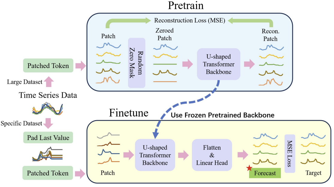
We have already seen that training models based on the Transformer architecture requires significant computational resources and a large training sample. Therefore, various pre-trained models are widely used when solving NLP and CV problems. Unfortunately, we do not have this opportunity when solving timeseries problems, because the nature and structure of timeseries is quite diverse. Understanding this, the authors of the U-shaped Transformer method propose dividing the model training process into 2 stages.

First, it is proposed to use a relatively large dataset to train the U-shaped Transformer model to restore randomly masked input data. This will allow the model to learn the structure of the input data, dependencies and context of the timeseries. Also, this will enable effective filtering of various noises. In addition, in their paper, the authors of the method supplemented the training dataset with data from various timeseries, which were collected not only in different time intervals, but from different sources. This is how they wanted to train the U-shaped Transformer to solve completely different problems.

In the second stage, the weights of the U-shaped Transformer are frozen. A decision-making "head" is added to it. It is fine-tuned to solve specific problems on a relatively small training dataset.

This addresses the problem of using 1 pre-trained U-shaped Transformer to solve several problems.

As you can see, fine-tuning is much faster and requires less resources compared to the full U-shaped Transformer training process.

Below is the general process as visualized by the authors.

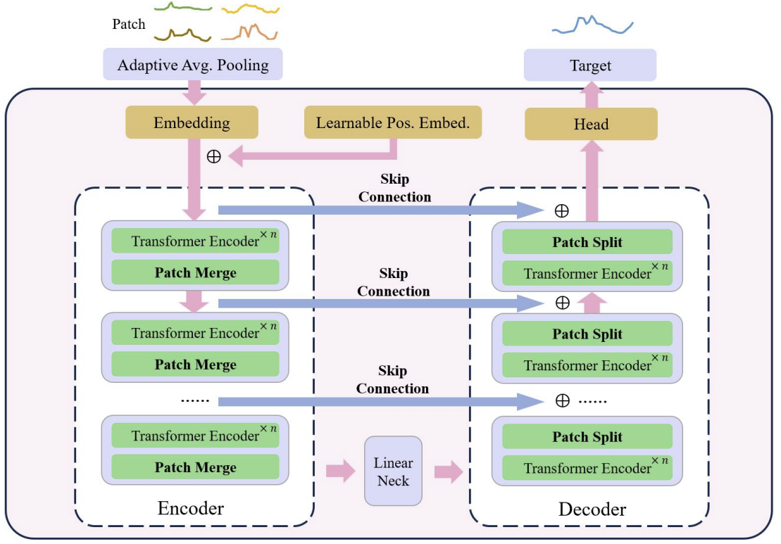
At the core of the U-shaped Transformer lies the stacking of Transformer layers. Several Transformer layers form a group. After processing the group, operations of merging or splitting patches are performed to integrate features of different scales.

Multiple skip-connections are used for fast data transfer from the encoder to the decoder. This allows high-frequency data to quickly approach the output of the neural network without unnecessary processing. Input data of the Transformer group are fed into the decoder output with the same shape. During the input data encoding process, as the model moves down, high-frequency features are continuously filtered out while common features are extracted. During the decoding process, the general features are continuously reconstructed with the detailed information from the skip-connection, which ultimately results in a temporal representation of the series combining both high-frequency and low-frequency features.

Patch operations are critical components for the U-shaped Transformer model as they enable the obtaining of features at different scales. The selected features directly affect the information that will be included in the underlying context of attention computation. Traditional approaches often split timeseries into dual arrays and treat them as independent channels. The authors of the U-shaped Transformer method consider this approach to be crude, since information about patches from different channels at one time step does not originate from neighboring regions. Therefore, they propose to use a convolution with a window size and stride of 2 as the patch pooling, which doubles the number of channels. This ensures that the previous patch is not fragmented and results in better merging of scales. During the decoding process, the authors of the method accordingly use transposed convolutions as a patch separation operation.

The U-shaped Transformer method uses convolution with a point kernel as an embedding method to map each patch to a higher-dimensional space. The authors of the method then prepare a trainable relative positional encoder for each patch, which is added to the embedding patches to enhance the accumulation of prior knowledge between patches.

As mentioned above, the U-shaped Transformer method authors use a patch-based embedding approach to split the timeseries data into smaller blocks. They use the patch recovery as the pre-task. The method authors believe that restoring unmasked patches can improve the model's robustness to noisy data with a value of zero.

After pre-training, the model is fine-tuned on a specific head unit, which is responsible for generating target tasks. At this stage, they freeze all components except the head networks.

To improve the generalization ability of the model and exploit the potential of the transformer on larger datasets, a larger dataset is used.

To further mitigate data imbalance, they use weighted random sampling, where the number of samples from different datasets during training is balanced.

To mitigate the problem of training instability in Transformer-based models, the authors of the method propose to normalize each mini-batch to bring the input data to a standard normal distribution. 

As a result, the proposed data preprocessing method achieves efficient feature extraction from different parts of the dataset and effectively overcomes the problem of data imbalance during joint training on multiple datasets.

2. Implementing in MQL5

After considering the theoretical aspects of the method, we move on to the practical part of our article, in which we implement the proposed approaches in MQL5.

As mentioned above, the U-shaped Transformer uses several architectural solutions that we will have to implement. Let's start with the block of trainable positional encoding.

2.1 Positional encoding

The positional encoding block is designed to enter information about the position of elements in a timeseries into the timeseries. As you know, the Self-Attention algorithm analyzes dependencies between elements regardless of their place in the series. But information about the position of an element in a series and about the distance between the analyzed elements can play an important role. This is especially true for time data series. To add this information, the classical Transformer uses the addition of a sinusoidal sequence to the input data. The periodicity of sinusoidal sequences is fixed and can vary in different implementations depending on the size of the sequence being analyzed.

Time series are characterized by the presence of some periodicity. Sometimes they have several frequency characteristics. In such cases, it is necessary to perform additional work to select the frequency characteristics of the positional coding tensor in such a way that it does not distort the original data or add extra information into them.

The original paper does not provide a detailed description of the method for the trainable positional encoding. I got the impression that the authors of the method selected a positional encoding coefficient for each element of the sequence during the model training process. Thus, it is fixed throughout the operation.

In our implementation, we will go a little further and make the positional coding coefficients dependent on the input data. We will use a simple fully connected layer to generate the positional encoding tensor. Naturally, we will train this layer during the learning process.

To implement the proposed mechanism, we will create a new class CNeuronLearnabledPE. As in most cases, we will inherit the main functionality from the neural layer base class CNeuronBaseOCL.

class CNeuronLearnabledPE  :  public CNeuronBaseOCL
  {
protected:
   CNeuronBaseOCL    cPositionEncoder;
   //---
   virtual bool      feedForward(CNeuronBaseOCL *NeuronOCL);
   virtual bool      updateInputWeights(CNeuronBaseOCL *NeuronOCL);
   virtual bool      calcInputGradients(CNeuronBaseOCL *NeuronOCL); 

public:
                     CNeuronLearnabledPE(void) {};
                    ~CNeuronLearnabledPE(void) {};
   //---
   virtual bool      Init(uint numOutputs, uint myIndex, COpenCLMy *open_cl, 
                          uint numNeurons, ENUM_OPTIMIZATION optimization_type, uint batch);
   //---
   virtual bool      Save(int const file_handle);
   virtual bool      Load(int const file_handle);
   //---
   virtual int       Type(void)        const                      {  return defNeuronLearnabledPE;    }
   virtual void      SetOpenCL(COpenCLMy *obj);
  };

The class structure has 1 nested object of the neural network base layer cPositionEncoder, which contains the trainable parameters of our positional coding tensor. This object is specified statically, and therefore we can leave the class constructor and destructor empty.

A class instance is initialized in the Init method. In the method parameters, we pass all the necessary information for the correct initialization of nested objects.

bool CNeuronLearnabledPE::Init(uint numOutputs, uint myIndex, COpenCLMy *open_cl, 
                               uint numNeurons, ENUM_OPTIMIZATION optimization_type, uint batch)
  {
   if(!CNeuronBaseOCL::Init(numOutputs, myIndex, open_cl, numNeurons, optimization_type, batch))
      return false;
   if(!cPositionEncoder.Init(0, 1, OpenCL, numNeurons, optimization, iBatch))
      return false;
   cPositionEncoder.SetActivationFunction(TANH);
   SetActivationFunction(None);
//---
   return true;
  }

The method algorithm is quite simple. In the body of the method, we first call the same method of the parent class, which checks the received external parameters and initializes the inherited objects. We determine the result of the operations by the logical value returned after executing the called method.

The next step is to initialize the nested cPositionEncoder object. For the nested object, we set the hyperbolic tangent as the activation function. The range of values of this function is from "-1" to "1", which corresponds to the range of values of sinusoidal wave sequences.

For our class of dynamic positional coding, there is no activation function.

After all iterations have successfully completed, we terminate the method with the true result.

Let's describe the feed-forward pass algorithm of our method in the CNeuronLearnabledPE::feedForward method. By analogy with the same method of the parent class, the method receives in parameters a pointer to the object of the previous neural layer, which contains the input data.

bool CNeuronLearnabledPE::feedForward(CNeuronBaseOCL *NeuronOCL)
  {
   if(!cPositionEncoder.FeedForward(NeuronOCL))
      return false;
   if(!SumAndNormilize(NeuronOCL.getOutput(), cPositionEncoder.getOutput(), Output, 1, false, 0, 0, 0, 1))
      return false;
//---
   return true;
  }

Based on the obtained initial data, we first generate a positional encoding tensor. Then we add the obtained values to the input data tensor.

The execution of all operations is controlled using the values returned by the called methods.

The CNeuronLearnabledPE::calcInputGradients algorithm of the error gradient distribution method looks a little more complicated. In the parameters, it also receives a pointer to the object of the previous neural layer, to which we must pass the error gradient.

bool CNeuronLearnabledPE::calcInputGradients(CNeuronBaseOCL *NeuronOCL)
  {
   if(!NeuronOCL)
      return false;
   if(!DeActivation(cPositionEncoder.getOutput(), cPositionEncoder.getGradient(), Gradient, 
                                                                      cPositionEncoder.Activation()))
      return false;
   if(!DeActivation(NeuronOCL.getOutput(), NeuronOCL.getGradient(), Gradient, NeuronOCL.Activation()))
      return false;
//---
   return true;
  }

In the method body, we first check the relevance of the pointer received in the parameters.

We then adjust the error gradient obtained from the subsequent layer to the activation function of the internal object. Let me remind you that during the initialization process, we specified an activation function for the internal object but left the CNeuronLearnabledPE object itself without an activation function. Therefore, the error gradient in our layer buffer was not corrected by the activation function.

The next step is to repeat the error gradient correction operation. However, this time we use it on the activation function of the previous layer.

Note that we do not propagate the error gradient through the internal object generating the positional encoding tensor. To execute the update of the parameters of this layer, we only need to have an error gradient at its output. We do not need to propagate the error gradient through the object to the previous layer, since the block generating the positional encoding tensor should not affect the input data or its embedding.

To complete the implementation of the backpropagation pass algorithm of the CNeuronLearnabledPE class, let's create a method to update the learning parameters: updateInputWeights. This method is very simplified: it calls the method of the nested object with the same name.

bool CNeuronLearnabledPE::updateInputWeights(CNeuronBaseOCL *NeuronOCL)
  {
   return cPositionEncoder.UpdateInputWeights(NeuronOCL);
  }

You can find the complete code of this class and all its methods in the attachment.

2.2 U-shaped Transformer class

Let's continue our version of the implementation of the approaches proposed by the authors of the U-shaped Transformer method. I must say that the decision on the implementation architecture for scip-connection between Encoder and Decoder, despite its apparent simplicity, turned out to be not so obvious. On one hand, we could use a reference to the inner layer identifier and pass data from the Encoder to the Decoder. There is nothing difficult here. But the question arises about the propagation of the error gradient through scip-connection. The entire backpropagation architecture of our classes is built on rewriting the error gradient during the subsequent backward pass. Therefore, any error gradient that we propagate through scip-connection will be removed during gradient propagation operations through neural layers between scip-connection objects.

As a solution, we can think of creating the whole U-shaped transformer architecture within one class. But we need a mechanism for constructing different numbers of Encoder-Decoder blocks with different numbers of Transformer layers in each block. The solution is the recurrent creation of objects. We will discuss the selected mechanism in more detail during the implementation process.

To implement our U-shaped Transformer block, we will create the CNeuronUShapeAttention class, which, like the previous one, will inherit the main functionality from the CNeuronBaseOCL neural layer base class.

class CNeuronUShapeAttention  :  public CNeuronBaseOCL
  {
protected:
   CNeuronMLMHAttentionOCL    cAttention[2];
   CNeuronConvOCL             cMergeSplit[2];
   CNeuronBaseOCL             *cNeck;
   //---
   virtual bool      feedForward(CNeuronBaseOCL *NeuronOCL);
   virtual bool      calcInputGradients(CNeuronBaseOCL *prevLayer);
   virtual bool      updateInputWeights(CNeuronBaseOCL *NeuronOCL);
   //---
public:
                     CNeuronUShapeAttention(void) {};
                    ~CNeuronUShapeAttention(void) { delete cNeck; }
   //---
   virtual bool      Init(uint numOutputs, uint myIndex, COpenCLMy *open_cl, uint window, uint window_key, 
                          uint heads, uint units_count, uint layers, uint inside_bloks, 
                          ENUM_OPTIMIZATION optimization_type, uint batch);
   //---
   virtual int       Type(void)   const   {  return defNeuronUShapeAttention;   }
   //--- methods for working with files
   virtual bool      Save(int const file_handle);
   virtual bool      Load(int const file_handle);
   virtual CLayerDescription* GetLayerInfo(void);
   virtual bool      WeightsUpdate(CNeuronBaseOCL *net, float tau);
   virtual void      SetOpenCL(COpenCLMy *obj);
  };

In the class body, we create an array of 2 elements of the multi-layer multi-headed attention class CNeuronMLMHAttentionOCL. These will be the Encoder and Decoder of the current block.

We also create an array of 2 convolutional layer elements, which we will use to work with patches.

All elements between the Encoder and Decoders of the current block are placed in the cNeck object of the neural layer base class, which in this case is dynamic. But how can an indefinite number of blocks be added into one block? To answer this question, I suggest moving on to considering the Init object initialization method.

As always, in the method parameters we receive the main constants of the object architecture:

• window — the size of the input data window (description vector of 1 element of the sequence)
• window_key — the size of the internal vector describing 1 element of a sequence in the Self-Attention Query, Key, Value entities
• heads — number of attention heads
• units_count — number of elements in the sequence
• layers — number of attention layers in one block
• inside_bloks — number of nested U-shaped Transformer blocks

Parameters window, window_key, heads and layers are used without changes for the current and nested U-shaped Transformer blocks.

bool CNeuronUShapeAttention::Init(uint numOutputs, uint myIndex, COpenCLMy *open_cl, uint window, uint window_key,
                                  uint heads, uint units_count, uint layers, uint inside_bloks, 
                                  ENUM_OPTIMIZATION optimization_type, uint batch)
  {
   if(!CNeuronBaseOCL::Init(numOutputs, myIndex, open_cl, window * units_count, optimization_type, batch))
      return false;

In the body of the method, we first call the same method of the parent class, which controls the received parameters and initializes the inherited objects.

Next, we initialize the Encoder and patch split objects.

   if(!cAttention[0].Init(0, 0, OpenCL, window, window_key, heads, units_count, layers, optimization, iBatch))
      return false;
   if(!cMergeSplit[0].Init(0, 1, OpenCL, 2 * window, 2 * window, 4 * window, (units_count + 1) / 2, 
                                                                                        optimization, iBatch))
      return false;

Next comes the most interesting block of the initialization method. We first check the number of specified nested blocks. If there are more than "0", then we create and initialize the U-shaped transformer nested block, similar to the current class. However, the number of elements in the sequence is increased by 2 times, which corresponds to the patch splitting result. We also decrease the number of nested blocks by "1".

   if(inside_bloks > 0)
     {
      CNeuronUShapeAttention *temp = new CNeuronUShapeAttention();
      if(!temp)
         return false;
      if(!temp.Init(0, 2, OpenCL, window, window_key, heads, 2 * units_count, layers, inside_bloks - 1, 
                                                                                      optimization, iBatch))
        {
         delete temp;
         return false;
        }
      cNeck = temp;
     }

We save the pointer to the created object in the cNeck variable. For this, we declared a dynamic object. Thus, by recurrently calling the initialization function, we create the required number of nested U-shaped Transformer groups.

In the last block, we create a convolutional layer of linear dependence between the Encoder and the Decoder.

     {
      CNeuronConvOCL *temp = new CNeuronConvOCL();
      if(!temp)
         return false;
      if(!temp.Init(0, 2, OpenCL, window, window, window, 2 * units_count, optimization, iBatch))
        {
         delete temp;
         return false;
        }
      cNeck = temp;
     }

Next, we initialize the Decoder and patch merge objects.

   if(!cAttention[1].Init(0, 3, OpenCL, window, window_key, heads, 2 * units_count, layers, optimization, iBatch))
      return false;
   if(!cMergeSplit[1].Init(0, 4, OpenCL, 2 * window, 2 * window, window, units_count, optimization, iBatch))
      return false;

To eliminate unnecessary copying operations, we replace the error gradient buffer.

   if(Gradient != cMergeSplit[1].getGradient())
      SetGradient(cMergeSplit[1].getGradient());
//---
   return true;
  }

Complete the method execution.

The feed-forward method which comes next is much simpler. In it, we only call the same-name methods of the internal layers one by one in accordance with the U-shaped Transformer algorithm. First, the input data passes through the Encoder block.

bool CNeuronUShapeAttention::feedForward(CNeuronBaseOCL *NeuronOCL)
  {
   if(!cAttention[0].FeedForward(NeuronOCL))
      return false;

Then we split patches.

   if(!cMergeSplit[0].FeedForward(cAttention[0].AsObject()))
      return false;

And we call the feed-forward method for nested blocks.

   if(!cNeck.FeedForward(cMergeSplit[0].AsObject()))
      return false;

The data processed in this way is fed to the Decoder.

   if(!cAttention[1].FeedForward(cNeck))
      return false;

Followed by the patch merging layer.

   if(!cMergeSplit[1].FeedForward(cAttention[1].AsObject()))
      return false;

Finally, we sum the results of the current U-shaped Transformer block with the received input data (scip-connection) to preserve the high-frequency signal.

   if(!SumAndNormilize(NeuronOCL.getOutput(), cMergeSplit[1].getOutput(), Output, 1, false))
      return false;
//---
   return true;
  }

Complete the method execution.

After implementing the feed-forward pass, we move on to creating the backpropagation methods. First, we create the error gradient propagation method CNeuronUShapeAttention::calcInputGradients, in the parameters of which we receive a pointer to the object of the previous layer, to which we must propagate the error gradient.

bool CNeuronUShapeAttention::calcInputGradients(CNeuronBaseOCL *prevLayer)
  {
   if(!prevLayer)
      return false;

In the method body, we immediately check the relevance of the received pointer.

Since we use replacement of data buffers, the error gradient is already stored in the nested patch merging layer buffer. So, we can call the corresponding error gradient distribution method.

   if(!cAttention[1].calcHiddenGradients(cMergeSplit[1].AsObject()))
      return false;

Next, we propagate the error gradient through the Decoder.

   if(!cNeck.calcHiddenGradients(cAttention[1].AsObject()))
      return false;

Then we sequentially pass the error gradient through the internal blocks of the U-shaped Transformer, the patch splitting layer and the Encoder.

   if(!cMergeSplit[0].calcHiddenGradients(cNeck.AsObject()))
      return false;
   if(!cAttention[0].calcHiddenGradients(cMergeSplit[0].AsObject()))
      return false;
   if(!prevLayer.calcHiddenGradients(cAttention[0].AsObject()))
      return false;

After that we sum the error gradients at the input and output of the current block (scip-connection).

   if(!SumAndNormilize(prevLayer.getGradient(), Gradient, prevLayer.getGradient(), 1, false))
      return false;
   if(!DeActivation(prevLayer.getOutput(), prevLayer.getGradient(), prevLayer.getGradient(), 
                                                                     prevLayer.Activation()))
      return false;
//---
   return true;
  }

Adjust the error gradient to the activation function of the previous layer and complete the method.

Error gradient propagation is followed by an adjustment of the model's trainable parameters. This functionality is implemented in the CNeuronUShapeAttention::updateInputWeights method. The method algorithm is quite simple. We just call the corresponding methods of the nested objects one by one.

bool CNeuronUShapeAttention::updateInputWeights(CNeuronBaseOCL *NeuronOCL)
  {
   if(!cAttention[0].UpdateInputWeights(NeuronOCL))
      return false;
   if(!cMergeSplit[0].UpdateInputWeights(cAttention[0].AsObject()))
      return false;
   if(!cNeck.UpdateInputWeights(cMergeSplit[0].AsObject()))
      return false;
   if(!cAttention[1].UpdateInputWeights(cNeck))
      return false;
   if(!cMergeSplit[1].UpdateInputWeights(cAttention[1].AsObject()))
      return false;
//---
   return true;
  }

Do not forget to control the results at each step.

Some more information should be provided regarding the file operation methods. The operations are rather simple in the CNeuronUShapeAttention::Save data saving method. We call the corresponding methods of the parent class and all nested objects one by one.

bool CNeuronUShapeAttention::Save(const int file_handle)
  {
   if(!CNeuronBaseOCL::Save(file_handle))
      return false;
   for(int i = 0; i < 2; i++)
     {
      if(!cAttention[i].Save(file_handle))
         return false;
      if(!cMergeSplit[i].Save(file_handle))
         return false;
     }
   if(!cNeck.Save(file_handle))
      return false;
//---
   return true;
  }

As for the data loading method CNeuronUShapeAttention::Load, there are some nuances. They are related to how loading of nested U-shaped Transformer blocks is organized. First, we call the parent class method to load the inherited objects.

bool CNeuronUShapeAttention::Load(const int file_handle)
  {
   if(!CNeuronBaseOCL::Load(file_handle))
      return false;

Then, in a loop, we load the Encoder, Decoder and Patch Layer data.

   for(int i = 0; i < 2; i++)
     {
      if(!LoadInsideLayer(file_handle, cAttention[i].AsObject()))
         return false;
      if(!LoadInsideLayer(file_handle, cMergeSplit[i].AsObject()))
         return false;
     }

Then we need to load nested blocks. As you remember, we use here a dynamic pointer to an object. Therefore, there are some options. The pointer in the variable may be invalid or it may point to an object of a different class.

We read the type of the required object from the file. We also check the type of the object that the cNeck variable points to. If the types differ, we delete the existing object.

   int type = FileReadInteger(file_handle);
   if(!!cNeck)
     {
      if(cNeck.Type() != type)
         delete cNeck;
     }

Next, we check the relevance of the pointer in the variable and, if necessary, create a new object of the appropriate type.

   if(!cNeck)
     {
      switch(type)
        {
         case defNeuronUShapeAttention:
            cNeck = new CNeuronUShapeAttention();
            if(!cNeck)
               return false;
            break;
         case defNeuronConvOCL:
            cNeck = new CNeuronConvOCL();
            if(!cNeck)
               return false;
            break;
         default:
            return false;
        }
     }

After completing the preparatory work, we load the object data from the file.

   cNeck.SetOpenCL(OpenCL);
   if(!cNeck.Load(file_handle))
      return false;

At the end of the method, we replace the error gradient buffers.

   if(Gradient != cMergeSplit[1].getGradient())
      SetGradient(cMergeSplit[1].getGradient());
//---
   return true;
  }

Complete the method execution.

You can find the full code of all classes and their methods, as well as all programs used in preparing the article, in the attachment.

2.3 Model architecture

After creating new classes for building our models, we move on to describing the architecture of the trainable models. For them, we create the file "...\Experts\UShapeTransformer\Trajectory.mqh".

AS mentioned earlier, the authors of the U-shaped Transformer method propose to train models in 2 steps. In the first step, we will train the Encoder to recover the masked data. Therefore, the description of the architecture of the Encoder model will be moved to a separate method called CreateEncoderDescriptions. In the method parameters, we pass a pointer to a dynamic array object for recording the description of the model architecture.

bool CreateEncoderDescriptions(CArrayObj *encoder)
  {
//---
   CLayerDescription *descr;
//---
   if(!encoder)
     {
      encoder = new CArrayObj();
      if(!encoder)
         return false;
     }

In the method body, we check the relevance of the received pointer and, if necessary, create a new instance of the dynamic array.

Next we create a source data layer of sufficient size.

//--- Encoder
   encoder.Clear();
//--- Input layer
   if(!(descr = new CLayerDescription()))
      return false;
   descr.type = defNeuronBaseOCL;
   int prev_count = descr.count = (HistoryBars * BarDescr);
   descr.activation = None;
   descr.optimization = ADAM;
   if(!encoder.Add(descr))
     {
      delete descr;
      return false;
     }

The input data is fed into the model in a "raw" form. Pre-process it in a batch normalization layer.

//--- layer 1
   if(!(descr = new CLayerDescription()))
      return false;
   descr.type = defNeuronBatchNormOCL;
   descr.count = prev_count;
   descr.batch = 1000;
   descr.activation = None;
   descr.optimization = ADAM;
   if(!encoder.Add(descr))
     {
      delete descr;
      return false;
     }

We save the batch normalization layer number to indicate it in the inverse normalization layer.

To train the Encoder, we use data masking. To perform masking, we create a Dropout layer.

//--- layer 2
   if(!(descr = new CLayerDescription()))
      return false;
   descr.type = defNeuronDropoutOCL;
   descr.count = prev_count;
   descr.probability = 0.4f;
   descr.activation = None;
   if(!encoder.Add(descr))
     {
      delete descr;
      return false;
     }

The masking probability is set to 0.4, which corresponds to 40% of the input data.

Please note that we are masking the original input data, not its embeddings.

In the next step, we use 2 convolutional layers to generate embeddings of the masked input data.

//--- layer 3
   if(!(descr = new CLayerDescription()))
      return false;
   descr.type = defNeuronConvOCL;
   prev_count = descr.count = HistoryBars;
   descr.window = BarDescr;
   descr.step = descr.window;
   int prev_wout = descr.window_out = EmbeddingSize / 2;
   if(!encoder.Add(descr))
     {
      delete descr;
      return false;
     }
//--- layer 4
   if(!(descr = new CLayerDescription()))
      return false;
   descr.type = defNeuronConvOCL;
   descr.count = prev_count;
   descr.window = prev_wout;
   descr.step = prev_wout;
   prev_wout = descr.window_out = EmbeddingSize;
   if(!encoder.Add(descr))
     {
      delete descr;
      return false;
     }

Then we add positional encoding to the input data. In this case, we use learnable positional encoding.

//--- layer 5
   if(!(descr = new CLayerDescription()))
      return false;
   descr.type = defNeuronLearnabledPE;
   descr.count = prev_count*prev_wout;
   if(!encoder.Add(descr))
     {
      delete descr;
      return false;
     }

Now we add the U-shaped Transformer block. The following parameters are used in the layer.

• descr.count: sequence size
• descr.window: size of vector of one element description
• descr.step: number of attention heads
• descr.window_out: size of the element of attention internal entities
• descr.layers: number of layers in each Transformer block
• descr.batch: number of nested U-shaped Transformer blocks

As you can see, most of the parameters have been taken from the attention blocks.

//--- layer 6
   if(!(descr = new CLayerDescription()))
      return false;
   descr.type = defNeuronUShapeAttention;
   descr.count = prev_count;
   descr.window = prev_wout;
   descr.step = 4;
   descr.window_out = EmbeddingSize;
   descr.layers = 3;
   descr.batch = 2;
   if(!encoder.Add(descr))
     {
      delete descr;
      return false;
     }

Next comes the decision-making block of 3 fully connected layers.

//--- layer 7
   if(!(descr = new CLayerDescription()))
      return false;
   descr.type = defNeuronBaseOCL;
   descr.count = LatentCount;
   descr.activation=SIGMOID;
   if(!encoder.Add(descr))
     {
      delete descr;
      return false;
     }
//--- layer 8
   if(!(descr = new CLayerDescription()))
      return false;
   descr.type = defNeuronBaseOCL;
   descr.count = LatentCount;
   descr.activation=LReLU;
   if(!encoder.Add(descr))
     {
      delete descr;
      return false;
     }
//--- layer 9
   if(!(descr = new CLayerDescription()))
      return false;
   descr.type = defNeuronBaseOCL;
   prev_count=descr.count = BarDescr*(HistoryBars+NForecast);
   descr.activation=TANH;
   if(!encoder.Add(descr))
     {
      delete descr;
      return false;
     }

Please note that at the output of the Encoder, we expect to receive the reconstructed input data plus several predicted values. In this way we want to train the U-shaped Transformer to capture dependencies not only in the input data, but also find reference points for constructing predicted values.

To complete the Encoder, we add a reverse normalization layer to make the reconstructed and predicted values comparable to the original input data.

//--- layer 10
   if(!(descr = new CLayerDescription()))
      return false;
   descr.type = defNeuronRevInDenormOCL;
   prev_count = descr.count = prev_count;
   descr.activation = None;
   descr.optimization = ADAM;
   descr.layers = 1;
   if(!encoder.Add(descr))
     {
      delete descr;
      return false;
     }
//---
   return true;
  }

Changing the Encoder architecture requires changing the hidden layer constant to obtain data from the model.

#define        LatentLayer             9

In addition, changing the size of the Encoder results layer also requires adjusting the architecture of the Actor and Critic models that use this data. The architecture of these models is provided in the CreateDescriptions method. In the parameters, the method receives pointers to 2 dynamic arrays for recording the architectures of the corresponding models.

bool CreateDescriptions(CArrayObj *actor, CArrayObj *critic)
  {
//---
   CLayerDescription *descr;
//---
   if(!actor)
     {
      actor = new CArrayObj();
      if(!actor)
         return false;
     }
   if(!critic)
     {
      critic = new CArrayObj();
      if(!critic)
         return false;
     }

In the method body, we check the received pointers and, if necessary, create new dynamic arrays.

First, we describe the Actor architecture. We feed the model with the account state description vector.

//--- Actor
   actor.Clear();
//--- Input layer
   if(!(descr = new CLayerDescription()))
      return false;
   descr.type = defNeuronBaseOCL;
   int prev_count = descr.count = AccountDescr;
   descr.activation = None;
   descr.optimization = ADAM;
   if(!actor.Add(descr))
     {
      delete descr;
      return false;
     }

The obtained data is processed by a fully connected layer.

//--- layer 1
   if(!(descr = new CLayerDescription()))
      return false;
   descr.type = defNeuronBaseOCL;
   prev_count = descr.count = EmbeddingSize;
   descr.activation = SIGMOID;
   descr.optimization = ADAM;
   if(!actor.Add(descr))
     {
      delete descr;
      return false;
     }

Next, we add 5 cross-attention layers, which will compare information about the account state and open positions with the data of the reconstructed and predicted values generated by the Encoder.

   for(int i = 0; i < 5; i++)
     {
      if(!(descr = new CLayerDescription()))
         return false;
      descr.type = defNeuronCrossAttenOCL;
        {
         int temp[] = {1, BarDescr};
         ArrayCopy(descr.units, temp);
        }
        {
         int temp[] = {EmbeddingSize, HistoryBars+NForecast};
         ArrayCopy(descr.windows, temp);
        }
      descr.window_out = 32;
      descr.step = 4;
      descr.activation = None;
      descr.optimization = ADAM;
      if(!actor.Add(descr))
        {
         delete descr;
         return false;
        }
     }

Note that we will not mask the input data at the Actor policy training and operation phases. However, it is expected that the trained Encoder will not only predict subsequent states of the environment, but also act as a kind of filter for historical values, removing various noises from them.

At the end of the model, there is a decision-making block with a stochastic "head".

//--- layer 8
   if(!(descr = new CLayerDescription()))
      return false;
   descr.type = defNeuronBaseOCL;
   descr.count = LatentCount;
   descr.activation = SIGMOID;
   descr.optimization = ADAM;
   if(!actor.Add(descr))
     {
      delete descr;
      return false;
     }
//--- layer 9
   if(!(descr = new CLayerDescription()))
      return false;
   descr.type = defNeuronBaseOCL;
   descr.count = 2 * NActions;
   descr.activation = None;
   descr.optimization = ADAM;
   if(!actor.Add(descr))
     {
      delete descr;
      return false;
     }
//--- layer 10
   if(!(descr = new CLayerDescription()))
      return false;
   descr.type = defNeuronVAEOCL;
   descr.count = NActions;
   descr.optimization = ADAM;
   if(!actor.Add(descr))
     {
      delete descr;
      return false;
     }

The Critic architecture has been adjusted accordingly. I will not describe these changes here. I suggest you familiarize yourself with them using codes provided in the attachment.

2.4 Encode Training EA

We have described the model architecture. Now let's move on to the Encoder model training EA. In this work, we use the training dataset collected for the previous article. In this dataset, we used a full array of historical data to describe the state of the environment. This approach has its pros and cons. The pros include the elimination of a stack inside the model for accumulating historical data and the ability to use sampled states to train models. However, the downside of it is the significant growth of the training dataset file as it contains data repeated many times. Also, during operation, the model at each step repeats the recalculation of historical data for the entire depth of the analyzed history. But at this stage, it is important to clearly compare the data fed to the model and the data restored after masking. Therefore, in order to test the proposed approaches, I decided to use this solution.

The new EA "...\Experts\UShapeTransformer\StudyEncoder.mq5" is mainly based on the relevant EA from the previous article. Therefore, we will not consider in detail all its methods. Let's consider the model training method: Train.

void Train(void)
  {
//---
   vector<float> probability = GetProbTrajectories(Buffer, 0.9);
//---
   vector<float> result, target;
   bool Stop = false;
//---
   uint ticks = GetTickCount();

At the beginning of the method, we do a little preparatory work. We define the probabilities of sampling trajectories based on their returns and declare local variables.

Then we organize a model training loop with the number of iterations specified by the user in the external parameters.

   for(int iter = 0; (iter < Iterations && !IsStopped() && !Stop); iter ++)
     {
      int tr = SampleTrajectory(probability);
      int i = (int)((MathRand() * MathRand() / MathPow(32767, 2)) * (Buffer[tr].Total - 2 - NForecast));
      if(i <= 0)
        {
         iter--;
         continue;
        }

In the body of the loop, we sample the trajectory and 1 state on it to train the model. We load information about the selected state into the data buffer.

      bState.AssignArray(Buffer[tr].States[i].state);
      //--- State Encoder
      if(!Encoder.feedForward((CBufferFloat*)GetPointer(bState), 1, false, (CBufferFloat*)NULL))
        {
         PrintFormat("%s -> %d", __FUNCTION__, __LINE__);
         Stop = true;
         break;
        }

Then we call the feed-forward pass method for our model, passing the loaded data to it.

After a successful execution of the feed-forward pass, the model's results buffer stores some representation of the historical environmental parameters and their predicted values. We are not interested in the specific result at the moment.

Now we need to prepare real data on the upcoming and analyzed environment states. As in the previous article, we first load subsequent environment states from the experience replay buffer.

      //--- Collect target data
      if(!Result.AssignArray(Buffer[tr].States[i + NForecast].state))
         continue;
      if(!Result.Resize(BarDescr * NForecast))
         continue;

Supplement them with data input into the model during the feed-forward pass. As we've seen, we have unmasked data in the buffer.

      if(!Result.AddArray(GetPointer(bState)))
         continue;

Now that we have prepared a buffer of target values, we can perform a backpropagation pass of the model and adjust the weights to minimize the error.

      if(!Encoder.backProp(Result, (CBufferFloat*)NULL))
        {
         PrintFormat("%s -> %d", __FUNCTION__, __LINE__);
         Stop = true;
         break;
        }

After updating the model parameters, we inform the user about the training progress and move on to the next iteration.

      if(GetTickCount() - ticks > 500)
        {
         double percent = double(iter) * 100.0 / (Iterations);
         string str = StringFormat("%-14s %6.2f%% -> Error %15.8f\n", "Encoder", percent, 
                                                                       Encoder.getRecentAverageError());
         Comment(str);
         ticks = GetTickCount();
        }
     }

Always make sure to check the operation execution result.

Once all iterations of the model training loop are successfully completed, we clear the comments field on the chart.

   Comment("");
//---
   PrintFormat("%s -> %d -> %-15s %10.7f", __FUNCTION__, __LINE__, "Encoder", Encoder.getRecentAverageError());
   ExpertRemove();
//---
  }

We output information about the model training results to the MetaTrader 5 log and initiate EA termination.

You can find the full code of the EA and all its methods in the attachment.

Actor and Critic policy training EA "...\Experts\RevIN\Study.mq5" has been copied from the previous article virtually unchanged. The same can be said about environmental interaction EAs. Therefore, we will not consider in detail their algorithms within this article. You can find the full code of all programs used in this article in the attachment.

I would like to emphasize once again that in all EAs, except for the Encoder training EA, the training mode must be disabled for the Encoder model.

   Encoder.TrainMode(false);

This will disable masking of the original input data.

3. Testing

We have discussed the theoretical aspects of the U-shaped Transformer method and done quite a lot of work on implementing the proposed approaches using MQL5. Now it's time to test the results of our work using real historical data.

As mentioned above, we will train the models using the training dataset collected for the previous article. We will not now consider a detailed description of the methods for collecting the training datasets as they were described in detail earlier.

The model is trained using historical data of EURUSD, H1, for 2023. The trained Actor policy is tested in the MetaTrader 5 strategy tester using historical data from January 2024, with the same symbol and timeframe.

In accordance with the approach proposed by the authors of the U-shaped Transformer method, we train models in 2 stages. First, we train the Encoder on pre-collected training data.

It should be noted here that the Encoder model analyzes only historical symbol data. Therefore, we do not need to collect additional passes during the Encoder training process. We can immediately set a sufficiently large number of model training iterations and wait for the training process to complete.

At this stage, I noticed a positive shift in the environment state forecasting quality.

The second stage of Actor policy learning is iterative. At this stage, we alternate Actor policy training with the collection of additional information about the environment by adding new passes to the training dataset using the EA "...\Experts\UShapeTransformer\Research.mq5" and the current Actor policy.

Through iterative learning, I was able to obtain a model capable of generating profit on both the training and testing datasets.

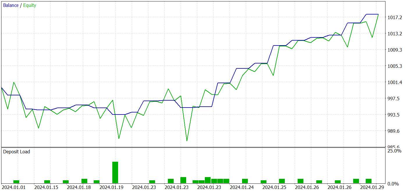
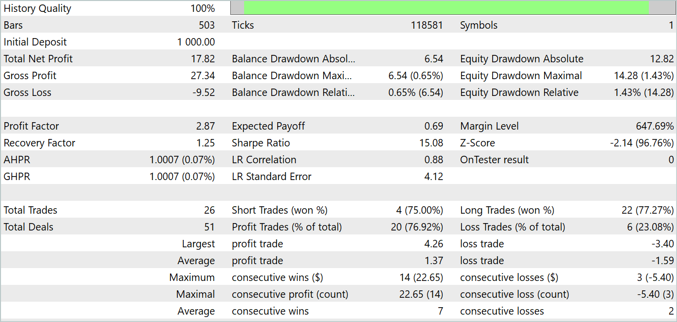
During the testing period, the model made 26 transactions. 20 of them were closed with a profit, which was 76.92%. The profit factor was 2.87.

The results obtained are promising, but the testing period of 1 month is too short to reliably assess the stability of the model.

Conclusion

In this article, we got acquainted with the U-shaped Transformer architecture, which was specifically designed for timeseries forecasting. The proposed approach combines the advantages of transformers and fully connected perceptrons, which allows effective capturing of long-term dependencies in time data and processing of high-frequency context.

One of the key achievements of U-shaped Transformer is the use of scip-connection and trainable patch merging and splitting operations. This allows the model to efficiently extract features across different scales and better capture information.

In the practical part of the article, we implemented the proposed approaches using MQL5. We trained and tested the resulting model using real historical data. We received quite good testing results.

However, once again, I would like to emphasize that all the programs presented in the article are intended only to demonstrate the technology and are not ready for use in real markets. The results of testing over a 1-month interval can only demonstrate the capabilities of the model but do not confirm its stable operation over a longer period of time.

References

U-shaped Transformer: Retain High Frequency Context in Time Series Analysis

Other articles from this series

Programs used in the article

#	Name	Type	Description
1	Research.mq5	EA	Example collection EA
2	ResearchRealORL.mq5	EA	EA for collecting examples using the Real-ORL method
3	Study.mq5	EA	Model training EA
4	StudyEncoder.mq5	EA	Encode training EA
5	Test.mq5	EA	Model testing EA
6	Trajectory.mqh	Class library	System state description structure
7	NeuroNet.mqh	Class library	A library of classes for creating a neural network
8	NeuroNet.cl	Code Base	OpenCL program code library