
Neural Networks Made Easy (Part 84): Reversible Normalization (RevIN)

Introduction
In the previous article, we discussed the Conformer method, which was originally developed for weather forecasting. This is quite an interesting method. When testing the trained model, we got a pretty good result. But did we do everything right? Is it possible to get a better result? Let's look at the learning process. We are clearly not using the model forecasting the next most probable timeseries values for its intended purpose. By feeding the model input data from a timeseries, we trained it by propagating the error gradient from models using the prediction results. We started with the Critic's results.
         if(!Critic.backProp(Result, (CNet *)GetPointer(Encoder)) ||
            !Encoder.backPropGradient((CBufferFloat*)NULL))
           {
            PrintFormat("%s -> %d", __FUNCTION__, __LINE__);
            Stop = true;
            break;
           }
Then Actor's results.
         if(!Actor.backProp(GetPointer(bActions), GetPointer(Encoder)) ||
            !Encoder.backPropGradient((CBufferFloat*)NULL))
           {
            PrintFormat("%s -> %d", __FUNCTION__, __LINE__);
            Stop = true;
            break;
           }
And once again data from the Actor, when adjusting its policy for the profitability of operations.
         Critic.TrainMode(false);
         if(!Critic.backProp(Result, (CNet *)GetPointer(Encoder)) ||
            !Actor.backPropGradient((CNet *)GetPointer(Encoder), -1, -1, false) ||
            !Encoder.backPropGradient((CBufferFloat*)NULL))
           {
            PrintFormat("%s -> %d", __FUNCTION__, __LINE__);
            Stop = true;
            break;
           }
There is nothing wrong with that, of course. It is a widely used practice in training various models. However, in this case, when training the Encoder model of the initial environment state, we focus not on predicting subsequent states, but on identifying individual features that allow us to optimize the operation of subsequent models.
Of course, our main task is to find the optimal policy of the Actor. So, at first glance, there is nothing wrong with adapting the Encoder model to the goals of the Actor. But in this case, the Encoder solves a slightly different problem. In practice, it becomes a block for subsequent models. Its architecture may not be optimal for solving the required tasks.
Moreover, when training the Encoder with error gradients of 3 different tasks, we may encounter a problem where the gradients of individual tasks are in different directions. In this case, the model will look for the "golden mean" that best satisfies all the tasks set. It is quite possible that such a solution may be quite far from optimal.
I think it is obvious that the structured logic of using models should also be implemented in the learning process. In such a paradigm, we need to train the Encoder to predict subsequent states of the environment. The Conformer approaches are used exactly in the Encoder. Then we train the Actor's policy taking into account the predicted states of the environment.
This is the theory, which is pretty clear. However, in practical implementation, we are faced with a significant gap in the distribution of individual features describing the state of the environment. Receiving such "raw" data describing the environment state at the input of the model, we normalize it to bring into a comparable form. But how do we get different values at the model output?
We have already encountered a similar problem when training various autoencoder models. In those cases, we found a solution in using the original data after normalization as targets. However, in this case we need data describing subsequent states of the environment that are different from the input data. One of the methods for solving this problem was proposed in the paper "Reversible Instance Normalization for Accurate Time-Series Forecasting against Distribution Shift".
The authors of the paper propose a simple yet effective normalization and denormalization method: Reversible Instantaneous Normalization (RevIN). The algorithm first normalizes the input sequences and then denormalizes the output sequences of the model to solve timeseries forecasting problems associated with distribution shift. RevIN is symmetrically structured to return the original distribution information to the model output by scaling and shifting the output in the denormalization layer in an amount equivalent to the shifting and scaling of the input data in the normalization layer.
RevIN is a flexible, trainable layer that can be applied to any arbitrarily chosen layers, effectively suppressing non-stationary information (mean and variance of an instance) in one layer and restoring it in another layer of nearly symmetric position, such as input and output layers.
1. RevIN Algorithm
To get acquainted with the RevIN algorithm, let's consider the problem of multivariate forecasting of timeseries in discrete time for a set of input data X = {xi}i=[1..N] and corresponding target Y = {yi}i=[1..N], where N denotes the number of elements in the sequence.
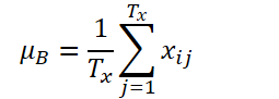
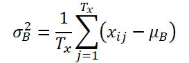
Let K, Txand Tydenote the number of variables, the length of the input sequence, and the length of the model prediction, respectively. Given the input sequence Xi∈ RK*Tx, our aim is to solve the time series forecasting problem, which is to predict the subsequent values Yi∈ RK*Ty. In RevIN, the length of input sequence Tx and the length of the forecast Ty may differ as observations are normalized and denormalized along the time dimension. The proposed method, RevIN, consists of symmetrically structured normalization and denormalization layers. First we normalize the input Xi using its mean and standard deviation, which is widely accepted as instant normalization. The mean and standard deviation are calculated for each input instance Xi as follows:

Normalized sequences can have more consistent mean and standard deviation, where non-stationary information is reduced. As a result, the normalization layer allows the model to accurately predict local dynamics within the sequence while receiving inputs of consistent distributions in terms of the mean and variance.
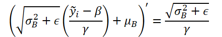
The model receives transformed data as input and predicts future values. However, the input data has different statistics compared to the original distribution, and by observing only the normalized input, it is difficult to capture the original distribution of the input data. Thus, to make this task easier for the model, we explicitly return the non-stationary features removed from the input data to the model output by reversing the normalization at a symmetric positioning, the output layer. The denormalization step can return the model output to the original timeseries value.. Accordingly, we denormalize the model output by applying the inverse normalization operation:

The same statistics used in the normalization step are used for scaling and shifting. Now ŷi is the final prediction of the model.
Simply added to virtually symmetrical positions in the network, RevIN can effectively reduce the distribution divergence ,in time-series data as the trainable normalization layer, generally applicable to arbitrary deep neural networks. Indeed, the proposed method is a flexible, learnable layer that can be applied to any arbitrarily selected layers, even to multiple layers. The authors of the method confirm its effectiveness as a flexible layer by adding it to intermediate layers in various models. Nevertheless, RevIN is most effective when applied to virtually symmetric layers of the Encoder-Decoder structure. In a typical time series forecasting model, the boundary between Encoder and Decoder is often unclear. Therefore, the authors of the method apply RevIN to the input and output layers of the model, since they can be viewed as an Encoder-Decoder structure that generates subsequent values based on the input data.
The original visualization of the RevIN method is presented below.

2. Implementing in MQL5
We have considered the theoretical aspects of the method. Now we can move on to the practical implementation of the proposed approaches using MQL5.
From the theoretical description of the method presented above, you can see that the normalization of the initial data proposed by the authors of the method completely repeats the algorithm of the CNeuronBatchNormOCL batch normalization layer that we implemented earlier. Therefore, we can use the existing class to normalize the data. But to denormalize the data, we need to create a new neural layer, CNeuronRevINDenormOCL.
2.1 Creating a new Denormalization layer
Obviously, the process of data denormalization will use the objects used in data normalization. That's why the new CNeuronRevINDenormOCL layer is derived from the CNeuronBatchNormOCL normalization layer.
class CNeuronRevINDenormOCL   :  public CNeuronBatchNormOCL
  {
protected:
   int               iBatchNormLayer;
   //---
   virtual bool      feedForward(CNeuronBaseOCL *NeuronOCL);
   virtual bool      updateInputWeights(CNeuronBaseOCL *NeuronOCL)   {  return true;   }

public:
                     CNeuronRevINDenormOCL(void)   :  iBatchNormLayer(-1) {};
                    ~CNeuronRevINDenormOCL(void) {};
   //---
   virtual bool      Init(uint numOutputs, uint myIndex, COpenCLMy *open_cl, uint numNeurons, int NormLayer,
                          CNeuronBatchNormOCL *normLayer);
   virtual int       GetNormLayer(void)   {  return iBatchNormLayer; }
   //---
   virtual bool      calcInputGradients(CNeuronBaseOCL *NeuronOCL);
   //---
   virtual bool      Save(int const file_handle);
   virtual bool      Load(int const file_handle);
   //---
   virtual int       Type(void)        const                      {  return defNeuronRevInDenormOCL;    }
   virtual CLayerDescription* GetLayerInfo(void);
   //---
   virtual bool      WeightsUpdate(CNeuronBaseOCL *source, float tau)   {  return true;   }
  };
According to the RevIN method algorithm, we should use parameters trained at the normalization stage fro denormalization. The logic here is that at the normalization stage we study the distribution of the input data. After that, we bring the input data into a comparable form, removing the "gaps". Then the model works with normalized data. At the output of the model, we denormalize the data, returning the distribution parameters of the input data. Thus, we expect the model output to contain predicted data in the "natural" distribution of the input data.
Obviously, at the denormalization step, the model parameters are not updated. Therefore, in the class structure we override the methods for updating the model parameters with "empty stubs". Nevertheless, we will have to implement the feed-forward pass algorithm and error gradient distribution. But first things first.
In this class we do not declare any additional internal objects. Therefore, the class constructor and destructor remain empty. However, we create a variable to store the normalization layer identifier in the model: iBatchNormLayer. Here we also create a public method to get the value of this variable: GetNormLayer(void).
The object of our new class is initialized in the CNeuronRevINDenormOCL::Init method. In the parameters, the method receives all the necessary information for successful initialization of internal objects and variables. It should be mentioned here that there is a very significant difference from similar methods of previously considered neural layers. In the parameters of the method, in addition to constants, we will pass a pointer to the object of the CNeuronBatchNormOCL batch normalization layer.
bool CNeuronRevINDenormOCL::Init(uint numOutputs, uint myIndex, COpenCLMy *open_cl, uint numNeurons,
                                 int NormLayer, CNeuronBatchNormOCL *normLayer)
  {
   if(NormLayer > 0)
     {
      if(!normLayer)
         return false;
      if(normLayer.Type() != defNeuronBatchNormOCL)
         return false;
      if(BatchOptions == normLayer.BatchOptions)
         BatchOptions = NULL;
      if(!CNeuronBatchNormOCL::Init(numOutputs, myIndex, open_cl, numNeurons, normLayer.iBatchSize, normLayer.Optimization()))
         return false;
      if(!!BatchOptions)
         delete BatchOptions;
      BatchOptions = normLayer.BatchOptions;
     }
Another fundamental difference lies in the body of the method. Here we create a branching algorithm depending on the received batch normalization layer identifier. If it is greater than 0, then we check the received pointer to the batch normalization layer. We also check the type of the received object. After that we call the same method of the parent class. Only after successfully passing all the specified control points, we replace the optimization parameter buffer.
Please note that we do not copy data. Instead, we completely change the pointer to the buffer object. Thus, during the model training process, we will work with always relevant normalization parameters.
The second branch of the algorithm is designed to initialize an empty class object during the process of loading a previously saved model. Here we just call the same parent class method with minimal parameters
   else
      if(!CNeuronBatchNormOCL::Init(numOutputs, myIndex, open_cl, numNeurons, 0, ADAM))
         return false;
Next, regardless of the chosen path, we save the obtained identifier of the batch normalization layer and complete the method.
   iBatchNormLayer = NormLayer;
//---
   return true;
  }
2.2 Organizing the feed-forward pass
We will start the implementation of the feed-forward pass algorithm by creating the RevInFeedForward kernel on the OpenCL program side. Similar to the implementation of the batch normalization layer algorithm, we will launch this kernel in a 1-dimensional task space.
In the kernel parameters, we will pass pointers to 3 data buffers: source data, normalization parameters and results. We will also pass 2 constants: the size of the buffer with normalization batch parameters and the parameter optimization type.
__kernel void RevInFeedForward(__global float *inputs, __global float *options,
                               __global float *output, int options_size,
                               int optimization)
  {
   int n = get_global_id(0);
Let me remind you that the size of the normalization parameter buffer depends on the selected parameter optimization algorithm. This buffer has the following structure.

In the kernel body, we identify the thread in the task space. We also determine the shift in the buffers till the analyzed data. In the source and result buffers, the offset is equal to the thread identifier. The shift in the optimization parameter buffer is determined in accordance with the given buffer structure and the specified parameter optimization method.
int shift = (n * optimization == 0 ? 7 : 9) % options_size;
In addition, here we must take into account that the number of environmental states analyzed may differ from the depth of our forecast. In this case, we should maintain the structure of the analyzed and predicted states of the environment. In other words, the number and order of the analyzed parameters of one environmental state description are completely preserved when predicting subsequent states. Thus, to determine the shift in the normalization parameter buffer, we take the remainder of dividing the shift calculated based on the analyzed thread and the buffer structure, by the size of the normalization parameter buffer.
The next step is to extract data from global buffers into local variables.
   float mean = options[shift];
   float variance = options[shift + 1];
   float k = options[shift + 3];
Calculate the denormalized value of the predicted parameter.
   float res = 0;
   if(k != 0)
      res = sqrt(variance) * (inputs[n] - options[shift + 4]) / k + mean;
   if(isnan(res))
      res = 0;
The result of the operations is written to the corresponding element of the result buffer.
   output[n] = res;
  }
After implementing the data denormalization algorithm on the OpenCL program side, we need to implement the created kernel call from the main program. For this, we need to override the CNeuronRevINDenormOCL::feedForward method.
bool CNeuronRevINDenormOCL::feedForward(CNeuronBaseOCL *NeuronOCL)
  {
   if(!OpenCL || !NeuronOCL)
      return false;
//---
   PrevLayer = NeuronOCL;
//---
   if(!BatchOptions)
      iBatchSize = 0;
   if(iBatchSize <= 1)
     {
      activation = (ENUM_ACTIVATION)NeuronOCL.Activation();
      return true;
     }
Like the same method of the parent class, this method will receive in parameters a pointer to the object of the previous layer, which contains the input data.
In the body of the method, we check the received pointer and save it in the corresponding variable.
Then we check the normalization batch size. And if it does not exceed "1", we consider this as no normalization and pass the data from the previous layer unchanged. Of course, we will not copy all the data. We will just copy the activation function identifier. When accessing the result or gradient buffer, we return pointers to the buffers of the previous layer. This functionality has already been implemented in the parent class.
Next, we implement the algorithm for directly placing the kernel in the execution queue. Here we first define the task space.
   uint global_work_offset[1] = {0};
   uint global_work_size[1] = {Neurons()};
After that we pass the necessary parameters to the kernel.
   ResetLastError();
   if(!OpenCL.SetArgumentBuffer(def_k_RevInFeedForward, def_k_revffinputs, NeuronOCL.getOutputIndex()))
     {
      printf("Error of set parameter kernel %s: %d; line %d", __FUNCTION__, GetLastError(), __LINE__);
      return false;
     }
   if(!OpenCL.SetArgumentBuffer(def_k_RevInFeedForward, def_k_revffoptions, BatchOptions.GetIndex()))
     {
      printf("Error of set parameter kernel %s: %d; line %d", __FUNCTION__, GetLastError(), __LINE__);
      return false;
     }
   if(!OpenCL.SetArgumentBuffer(def_k_RevInFeedForward, def_k_revffoutput, Output.GetIndex()))
     {
      printf("Error of set parameter kernel %s: %d; line %d", __FUNCTION__, GetLastError(), __LINE__);
      return false;
     }
   if(!OpenCL.SetArgument(def_k_RevInFeedForward, def_k_revffoptions_size, (int)BatchOptions.Total()))
     {
      printf("Error of set parameter kernel %s: %d; line %d", __FUNCTION__, GetLastError(), __LINE__);
      return false;
     }
   if(!OpenCL.SetArgument(def_k_RevInFeedForward, def_k_revffoptimization, (int)optimization))
     {
      printf("Error of set parameter kernel %s: %d; line %d", __FUNCTION__, GetLastError(), __LINE__);
      return false;
     }
Send the kernel to the execution queue.
   if(!OpenCL.Execute(def_k_RevInFeedForward, 1, global_work_offset, global_work_size))
     {
      printf("Error of execution kernel %s: %d", __FUNCTION__, GetLastError());
      return false;
     }
//---
   return true;
  }
Do not forget to control operations at each step.
2.3 Error Gradient Propagation Algorithm
After implementing the feed-forward pass, we need to implement the backpropagation algorithm. As mentioned above, this layer does not contain any learnable parameters. It uses the parameters trained during the normalization stage. Therefore, all parameter updating methods are replaced with "stubs".
However, the layer participates in backpropagation algorithms and the error gradient is propagated through it to the previous neural layer. As before, we first create the RevInHiddenGradient kernel on the side of the OpenCL program. This time the number of kernel parameters has increased. We pass 4 pointers to data buffers: buffers for results and error gradients of the previous layer, optimization parameters and the error gradient at the current layer results layer. We also pass 3 constants: the size of the normalization parameter buffer, the parameter optimization type, and the activation function of the previous layer.
__kernel void RevInHiddenGraddient(__global float *inputs, __global float *inputs_gr,
                                   __global float *options, __global float *output_gr,
                                   int options_size,
                                   int optimization,
                                   int activation)
  {
   int n = get_global_id(0);
   int shift = (n * optimization == 0 ? 7 : 9) % options_size;
In the kernel body, we first identify the thread and determine shifts in the data buffers. The algorithm for determining the shift in buffers is described above in the part related to the feed-forward kernel.
Next, we load data from global data buffers into local variables.
   float variance = options[shift + 1];
   float inp = inputs[n];
   float k = options[shift + 3];
Then we adjust the error gradient by the derivative of the denormalization function. It should be noted here that at the denormalization stage, all normalization parameters are constants, while the derivative of the function is significantly simplified.
Let's implement the presented function in code.
   float res = 0;
   if(k != 0)
      res = sqrt(variance) * output_gr[n] / k;
   if(isnan(res))
      res = 0;
After that, we adjust the error gradient by the derivative of the activation function of the previous neural layer.
   switch(activation)
     {
      case 0:
         res = clamp(res + inp, -1.0f, 1.0f) - inp;
         res = res * (1 - pow(inp == 1 || inp == -1 ? 0.99999999f : inp, 2));
         break;
      case 1:
         res= clamp(res + inp, 0.0f, 1.0f) - inp;
         res = res * (inp == 0 || inp == 1 ? 0.00000001f : (inp * (1 - inp)));
         break;
      case 2:
         if(inp < 0)
            res *= 0.01f;
         break;
      default:
         break;
     }
Save the result of the operations in the corresponding element of the error gradient buffer of the previous neural layer.
//---
   inputs_gr[n] = res;
  }
The next step is to implement the kernel call on the main program side. This functionality is implemented in the CNeuronRevINDenormOCL::calcInputGradients method. The algorithm for placing the kernel in the execution queue is the same as the one described above for the feed-forward method. Therefore, we will not discuss it in detail now.
Also, we won't consider auxiliary methods of the class. Their algorithm is quite simple, so you can study it yourself using the attached files. Also, the attachment contains the full code of all methods of the new class and previously created ones. So, you can study all the programs used in the article.
2.4 Spot edits in higher level classes
A few words should be said about making specific edits to the methods of higher-level classes, which are caused by the specifics of our new CNeuronRevINDenormOCL class. This concerns the initialization and loading of objects of this class.
When describing the method of initializing an object of our CNeuronRevINDenormOCL class, we mentioned the peculiarity of passing a pointer to a data normalization layer object. Note that at the time of describing the model architecture, we do not have a pointer to this object for one simple reason – this object has not yet been created. We can only indicate the ordinal number of the layer, which we know from the described architecture of the model.
However, we clearly know that the normalization layer comes before the denormalization layer. Furthermore, there can be an arbitrary number of neural layers between them. This means that at the time of creating the denormalization layer object, a normalization layer must already be created in the model. We can access it, but only inside the model. Because access to individual neural layers is closed to external programs.
Therefore, in the CNet::Create method, we create a separate block to initialize the CNeuronRevINDenormOCL denormalization layer object.
            case defNeuronRevInDenormOCL:
               if(desc.layers>=layers.Total())
                 {
                  delete temp;
                  return false;
                 }
Here we first check that a layer with the specified identifier has already been created in our model.
Then we check the type of the specified layer. It should be a batch normalization layer.
               if(((CLayer *)layers.At(desc.layers)).At(0).Type()!=defNeuronBatchNormOCL)
                 {
                  delete temp;
                  return false;
                 }
Only after the specified controls are successfully passed, we create a new object.
               revin = new CNeuronRevINDenormOCL();
               if(!revin)
                 {
                  delete temp;
                  return false;
                 }
Initialize it.
               if(!revin.Init(outputs, 0, opencl, desc.count, desc.layers,
                                  ((CLayer *)layers.At(desc.layers)).At(0)))
                 {
                  delete temp;
                  delete revin;
                  return false;
                 }
Add it to the array of objects.
               if(!temp.Add(revin))
                 {
                  delete temp;
                  delete revin;
                  return false;
                 }
               break;
In addition, there is a nuance when loading a previously trained model. As you know, in the initialization method of our new class, we created a branching algorithm depending on the identifier of the normalization layer. This was done to enable loading a pre-trained model. The point is that before loading an object we need to create a "blank" of it. This functionality is performed in the CLayer::CreateElement method. The difficulty is that before loading the data, we don't yet know the identifier of the normalization layer. That's why we specify "-1" as the identifier and "NULL" as the object pointer.
         case  defNeuronRevInDenormOCL:
            if(CheckPointer(OpenCL) == POINTER_INVALID)
               return false;
            revin = new CNeuronRevINDenormOCL();
            if(CheckPointer(revin) == POINTER_INVALID)
               result = false;
            if(revin.Init(iOutputs, index, OpenCL, 1, -1, NULL))
              {
               m_data[index] = revin;
               return true;
              }
            delete revin;
            break;
Then, during the loading process, all the data is loaded into the internal objects and variables of our class. But there is a nuance here too. During the data loading process, we get the normalization parameters saved after pre-training the model. But we don't need this. To train and operate the model further, we need to synchronize parameters between the normalization and denormalization layers. Otherwise, we would have a gap between the distributions of the input data and our forecasts. Therefore, we go to the CNet::Load method and after loading the next neural layer, we check its type.
bool CNet::Load(const int file_handle)
  {
........
........
//--- read array length
   num = FileReadInteger(file_handle, INT_VALUE);
//--- read array
   if(num != 0)
     {
      for(i = 0; i < num; i++)
        {
         //--- create new element
         CLayer *Layer = new CLayer(0, file_handle, opencl);
         if(!Layer.Load(file_handle))
            break;
         if(Layer.At(0).Type() == defNeuronRevInDenormOCL)
           {
            CNeuronRevINDenormOCL *revin = Layer.At(0);
            int l = revin.GetNormLayer();
            if(!layers.At(l))
              {
               delete Layer;
               break;
              }
If the CNeuronRevINDenormOCL denormalization layer is detected, we request a pointer to the normalization layer and check if such a layer is loaded.
We also check the type of this layer.
            CNeuronBaseOCL *neuron = ((CLayer *)layers.At(l)).At(0);
            if(neuron.Type() != defNeuronBatchNormOCL)
              {
               delete Layer;
               break;
              }
Once the specified control points are successfully passed, we initialize the layer object by passing a pointer to the corresponding normalization layer.
            if(!revin.Init(revin.getConnections(), 0, opencl, revin.Neurons(), l, neuron))
              {
               delete Layer;
               break;
              }
           }
         if(!layers.Add(Layer))
            break;
        }
     }
   FileClose(file_handle);
//--- result
   return (layers.Total() == num);
  }
Then we follow the previously created algorithm.
You can find the full code of all classes and their methods, as well as all programs used in preparing the article, in the attachment.
2.5 Model architecture for training
We have implemented the approaches proposed by the authors of the RevIN method using MQL5. Now it's time to include them into the architecture of our models. As discussed earlier, we will use denormalization in the Encoder model in order to implement the ability to train it to predict subsequent states of the environment. We will define the number of forecast states of the environment (in our case, subsequent candles) in the NForecast constant.
#define NForecast 6 //Number of forecast
Since we plan to train the Encoder separately from the Actor and Critic, we will also move the description of the Encoder architecture into a separate method, CreateEncoderDescriptions. In the parameters to the method, we will pass only one pointer to a dynamic array to save the architecture of the created model. It should be noted here that our implementation of the CNeuronRevINDenormOCL class does not allow the Decoder to be allocated as a separate model.
bool CreateEncoderDescriptions(CArrayObj *encoder)
  {
//---
   CLayerDescription *descr;
//---
   if(!encoder)
     {
      encoder = new CArrayObj();
      if(!encoder)
         return false;
     }
In the body of the method, we check the received pointer and, if necessary, create a new instance of the dynamic array object.
As before, we feed the model with "raw" input data describing the state of the environment.
//--- Encoder
   encoder.Clear();
//--- Input layer
   if(!(descr = new CLayerDescription()))
      return false;
   descr.type = defNeuronBaseOCL;
   int prev_count = descr.count = (HistoryBars * BarDescr);
   descr.activation = None;
   descr.optimization = ADAM;
   if(!encoder.Add(descr))
     {
      delete descr;
      return false;
     }
The received data undergoes primary processing in the batch normalization layer. We need to save the ordinal number of the layer.
//--- layer 1
   if(!(descr = new CLayerDescription()))
      return false;
   descr.type = defNeuronBatchNormOCL;
   descr.count = prev_count;
   descr.batch = MathMax(1000, GPTBars);
   descr.activation = None;
   descr.optimization = ADAM;
   if(!encoder.Add(descr))
     {
      delete descr;
      return false;
     }
After normalizing the input data, we create the data embedding and add it to the internal stack.
//--- layer 2
   if(!(descr = new CLayerDescription()))
      return false;
   descr.type = defNeuronEmbeddingOCL;
     {
      int temp[] = {4, 1, 1, 1, 2};
      ArrayCopy(descr.windows, temp);
     }
   prev_count = descr.count = GPTBars;
   int prev_wout = descr.window_out = EmbeddingSize / 2;
   if(!encoder.Add(descr))
     {
      delete descr;
      return false;
     }
//--- layer 3
   if(!(descr = new CLayerDescription()))
      return false;
   descr.type = defNeuronConvOCL;
   descr.count = prev_count * 5;
   descr.step = descr.window = prev_wout;
   prev_wout = descr.window_out = EmbeddingSize;
   if(!encoder.Add(descr))
     {
      delete descr;
      return false;
     }
Then we add positional encoding of the data.
//--- layer 4
   if(!(descr = new CLayerDescription()))
      return false;
   descr.type = defNeuronPEOCL;
   descr.count = prev_count;
   descr.window = prev_wout * 5;
   if(!encoder.Add(descr))
     {
      delete descr;
      return false;
     }
We feed the prepared data into the 5-layer CNeuronConformer block.
//--- layer 5-10
   for(int i = 0; i < 5; i++)
     {
      if(!(descr = new CLayerDescription()))
         return false;
      descr.type = defNeuronConformerOCL;
      descr.count = prev_count;
      descr.window = prev_wout;
      descr.step = 4;
      descr.window_out = EmbeddingSize;
      descr.layers = 5;
      if(!encoder.Add(descr))
        {
         delete descr;
         return false;
        }
     }
To test the method, we use a fully connected layer with an appropriate number of elements as a decoder. However, to improve the quality of prediction, it is recommended to use a Decoder with a more complex architecture.
//--- layer 11
   if(!(descr = new CLayerDescription()))
      return false;
   descr.type = defNeuronBaseOCL;
   prev_count = descr.count = NForecast*BarDescr;
   descr.activation = TANH;
   descr.optimization = ADAM;
   if(!encoder.Add(descr))
     {
      delete descr;
      return false;
     }
We are working with normalized data and assume that its variance is close to 1 and its mean is close to 0. Therefore, we use the hyperbolic tangent (tanh) as the activation function at the Decoder output. As you know, the range of its values is from "-1" to "1".
And finally, we denormalize the forecast values.
//--- layer 12
   if(!(descr = new CLayerDescription()))
      return false;
   descr.type = defNeuronRevInDenormOCL;
   prev_count = descr.count = prev_count;
   descr.activation = None;
   descr.optimization = ADAM;
   descr.layers=1;
   if(!encoder.Add(descr))
     {
      delete descr;
      return false;
     }
//---
   return true;
  }
To complete the work on describing the architecture of the models, let's consider the construction of the Actor and the Critic. The architecture of the specified models is described in the CreateDescriptions method. It is very similar to the one described in the previous article, but there is a nuance.
In the parameters, the method receives pointers to 2 dynamic arrays.
bool CreateDescriptions(CArrayObj *actor, CArrayObj *critic)
  {
//---
   CLayerDescription *descr;
//---
   if(!actor)
     {
      actor = new CArrayObj();
      if(!actor)
         return false;
     }
   if(!critic)
     {
      critic = new CArrayObj();
      if(!critic)
         return false;
     }
In the body of the method, we check the received pointers and, if necessary, create new object instances.
We feed the Actor a tensor describing the account status and open positions.
//--- Actor
   actor.Clear();
//--- Input layer
   if(!(descr = new CLayerDescription()))
      return false;
   descr.type = defNeuronBaseOCL;
   int prev_count = descr.count = AccountDescr;
   descr.activation = None;
   descr.optimization = ADAM;
   if(!actor.Add(descr))
     {
      delete descr;
      return false;
     }
Generate an embedding of this representation.
//--- layer 1
   if(!(descr = new CLayerDescription()))
      return false;
   descr.type = defNeuronBaseOCL;
   prev_count = descr.count = EmbeddingSize;
   descr.activation = SIGMOID;
   descr.optimization = ADAM;
   if(!actor.Add(descr))
     {
      delete descr;
      return false;
     }
Then comes the Cross-Attention block, which analyzes the current state of the account against the predicted states of the environment.
//--- layer 2-4
   for(int i = 0; i < 3; i++)
     {
      if(!(descr = new CLayerDescription()))
         return false;
      descr.type = defNeuronCrossAttenOCL;
        {
         int temp[] = {1, NForecast};
         ArrayCopy(descr.units, temp);
        }
        {
         int temp[] = {EmbeddingSize, BarDescr};
         ArrayCopy(descr.windows, temp);
        }
      descr.window_out = 16;
      descr.step = 4;
      descr.activation = None;
      descr.optimization = ADAM;
      if(!actor.Add(descr))
        {
         delete descr;
         return false;
        }
     }
At the end of the Actor model there is a decision-making block with a stochastic policy.
//--- layer 5
   if(!(descr = new CLayerDescription()))
      return false;
   descr.type = defNeuronBaseOCL;
   descr.count = LatentCount;
   descr.activation = SIGMOID;
   descr.optimization = ADAM;
   if(!actor.Add(descr))
     {
      delete descr;
      return false;
     }
//--- layer 6
   if(!(descr = new CLayerDescription()))
      return false;
   descr.type = defNeuronBaseOCL;
   descr.count = 2 * NActions;
   descr.activation = None;
   descr.optimization = ADAM;
   if(!actor.Add(descr))
     {
      delete descr;
      return false;
     }
//--- layer 7
   if(!(descr = new CLayerDescription()))
      return false;
   descr.type = defNeuronVAEOCL;
   descr.count = NActions;
   descr.optimization = ADAM;
   if(!actor.Add(descr))
     {
      delete descr;
      return false;
     }
The Critic model is constructed in a similar way. Only instead of describing the account state, the Critic analyzes the Actor's actions in the context of the predicted states of the environment.
//--- Critic
   critic.Clear();
//--- Input layer
   if(!(descr = new CLayerDescription()))
      return false;
   descr.type = defNeuronBaseOCL;
   prev_count = descr.count = NActions;
   descr.activation = None;
   descr.optimization = ADAM;
   if(!critic.Add(descr))
     {
      delete descr;
      return false;
     }
//--- layer 1
   if(!(descr = new CLayerDescription()))
      return false;
   descr.type = defNeuronBaseOCL;
   prev_count = descr.count = EmbeddingSize;
   descr.activation = SIGMOID;
   descr.optimization = ADAM;
   if(!critic.Add(descr))
     {
      delete descr;
      return false;
     }
//--- layer 2-4
   for(int i = 0; i < 3; i++)
     {
      if(!(descr = new CLayerDescription()))
         return false;
      descr.type = defNeuronCrossAttenOCL;
        {
         int temp[] = {1, NForecast};
         ArrayCopy(descr.units, temp);
        }
        {
         int temp[] = {EmbeddingSize, BarDescr};
         ArrayCopy(descr.windows, temp);
        }
      descr.window_out = 16;
      descr.step = 4;
      descr.activation = None;
      descr.optimization = ADAM;
      if(!critic.Add(descr))
        {
         delete descr;
         return false;
        }
     }
//--- layer 5
   if(!(descr = new CLayerDescription()))
      return false;
   descr.type = defNeuronBaseOCL;
   descr.count = LatentCount;
   descr.activation = SIGMOID;
   descr.optimization = ADAM;
   if(!critic.Add(descr))
     {
      delete descr;
      return false;
     }
//--- layer 6
   if(!(descr = new CLayerDescription()))
      return false;
   descr.type = defNeuronBaseOCL;
   descr.count = LatentCount;
   descr.activation = SIGMOID;
   descr.optimization = ADAM;
   if(!critic.Add(descr))
     {
      delete descr;
      return false;
     }
//--- layer 7
   if(!(descr = new CLayerDescription()))
      return false;
   descr.type = defNeuronBaseOCL;
   descr.count = NRewards;
   descr.activation = None;
   descr.optimization = ADAM;
   if(!critic.Add(descr))
     {
      delete descr;
      return false;
     }
//---
   return true;
  }
At the output of the Critic we get a clear, not stochastic, assessment of the Agent's actions.
2.6 Model training programs
After describing the architecture of the trained models, we move on to creating programs to train them. To train the Encoder, we will create an Expert Advisor: "...\Experts\RevIN\StudyEncoder.mq5". The EA architecture follows those from previous articles. So, we have already discussed it multiple times within this series. Therefore, we will only focus on the model training method Train.
void Train(void)
  {
//---
   vector<float> probability = GetProbTrajectories(Buffer, 0.9);
//---
   vector<float> result, target;
   bool Stop = false;
//---
   uint ticks = GetTickCount();
In the body of the method, as usual, we generate a vector of probabilities of choosing trajectories depending on their profitability. For future environmental state prediction, all passes are the same. Because the Encoder does not analyze account status and open positions. However, we do not remove this functionality in case there is an experience replay buffer based on the passes at different historical intervals.
Then we prepare local variables and organize a system of model training loops.
   for(int iter = 0; (iter < Iterations && !IsStopped() && !Stop); iter ++)
     {
      int tr = SampleTrajectory(probability);
      int batch = GPTBars + 48;
      int state = (int)((MathRand() * MathRand() / MathPow(32767, 2)) * (Buffer[tr].Total - 2 - NForecast - batch));
      if(state <= 0)
        {
         iter--;
         continue;
        }
      Encoder.Clear();
      int end = MathMin(state + batch, Buffer[tr].Total - NForecast);
In the body of the outer loop, we sample the trajectory from the experience replay buffer and the state of the start of learning on it. We then determine the final state of the training batch and clear the internal model stack. After that, we run a nested learning cycle for the selected segment of historical data.
      for(int i = state; i < end && !IsStopped() && !Stop; i++)
        {
         bState.AssignArray(Buffer[tr].States[i].state);
         //--- State Encoder
         if(!Encoder.feedForward((CBufferFloat*)GetPointer(bState), 1, false, (CBufferFloat*)NULL))
           {
            PrintFormat("%s -> %d", __FUNCTION__, __LINE__);
            Stop = true;
            break;
           }
Here we first load the desired state from the training set. We move it to the data buffer. Then we execute a feed-forward pass of the Encoder by calling the corresponding method of our model.
In the next step, we prepare the target data. To do this, we organize another nested loop in which we take the required number of subsequent states from the training sample and add them to the data buffer.
         //--- Collect target data
         bState.Clear();
         for(int fst = 1; fst <= NForecast; fst++)
           {
            if(!bState.AddArray(Buffer[tr].States[i + fst].state))
               break;
           }
After collecting the target values, we can run the Encoder backpropagation pass to minimize the error between the predicted and target values.
         if(!Encoder.backProp(GetPointer(bState), (CBufferFloat*)NULL))
           {
            PrintFormat("%s -> %d", __FUNCTION__, __LINE__);
            Stop = true;
            break;
           }
Then we inform the user about the training progress and move on to the next training iteration.
         if(GetTickCount() - ticks > 500)
           {
            double percent = (double(i - state) / ((end - state)) + iter) * 100.0 / (Iterations);
            string str = StringFormat("%-14s %6.2f%% -> Error %15.8f\n", "Encoder", percent,
                                                                          Encoder.getRecentAverageError());
            Comment(str);
            ticks = GetTickCount();
           }
        }
     }
After all training iterations have successfully completed, we clear the comment field.
   Comment("");
//---
   PrintFormat("%s -> %d -> %-15s %10.7f", __FUNCTION__, __LINE__, "Encoder", Encoder.getRecentAverageError());
   ExpertRemove();
//---
  }
We output information about the achieved training results to the log and initialize the EA termination.
Training a model to predict future states of the environment is useful. However, our goal is to train the Actor policy. In the next step, we create the Actor and Critic training EA "...\Experts\RevIN\Study.mq5". The advisor is constructed based on the same architecture, so we will only touch on specific changes.
First, during the EA initialization, if there is no pre-trained Encoder, we generate an error of incorrect program initialization.
int OnInit()
  {
//---
........
........
//--- load models
   float temp;
   if(!Encoder.Load(FileName + "Enc.nnw", temp, temp, temp, dtStudied, true))
     {
      PrintFormat("Error of load Encoder: %d", GetLastError());
      return INIT_FAILED;
     }
........
........
//---
   return(INIT_SUCCEEDED);
  }
Second, the Encoder in this model is not trained and, accordingly, should not be saved.
void OnDeinit(const int reason)
  {
//---
   if(!(reason == REASON_INITFAILED || reason == REASON_RECOMPILE))
     {
      Actor.Save(FileName + "Act.nnw", 0, 0, 0, TimeCurrent(), true);
      Critic.Save(FileName + "Crt.nnw", 0, 0, 0, TimeCurrent(), true);
     }
   delete Result;
   delete OpenCL;
  }
Additionally, there is one thing when using the Encoder as the source of input data for the Actor and Critic. At the beginning of the article, we talked about the importance of using normalized data to train and operate models. The Denormalization layer at the Encoder output, on the other hand, returns our predictions to the original data distribution, making them incomparable.
However, we have long ago implemented the functionality of accessing the hidden layers of the model to extract data. So, we will use this functionality to obtain normalized predicted data from the penultimate layer of the Encoder. It is this data that we will use as the initial data for the Actor and Critic. We specify the pointer to the required layer in the LatentLayer constant.
#define LatentLayer 11
The feed-forward call for the Critic can look like:
         if(!Critic.feedForward((CBufferFloat*)GetPointer(bActions), 1, false, GetPointer(Encoder),LatentLayer))
           {
            PrintFormat("%s -> %d", __FUNCTION__, __LINE__);
            Stop = true;
            break;
           }
or
         if(!Critic.feedForward((CNet *)GetPointer(Actor), -1, (CNet*)GetPointer(Encoder),LatentLayer))
           {
            PrintFormat("%s -> %d", __FUNCTION__, __LINE__);
            Stop = true;
            break;
           }
Accordingly, we write the Actor's feed-forward call as
         if(!Actor.feedForward((CBufferFloat*)GetPointer(bAccount), 1, false, GetPointer(Encoder),LatentLayer))
           {
            PrintFormat("%s -> %d", __FUNCTION__, __LINE__);
            Stop = true;
            break;
           }
Don't forget to specify the layer identifier when calling the backpropagation methods of our models.
         if(!Critic.backProp(Result, (CNet *)GetPointer(Encoder),LatentLayer))
           {
            PrintFormat("%s -> %d", __FUNCTION__, __LINE__);
            Stop = true;
            break;
           }
         if(!Actor.backProp(GetPointer(bActions), GetPointer(Encoder),LatentLayer))
           {
            PrintFormat("%s -> %d", __FUNCTION__, __LINE__);
            Stop = true;
            break;
           }
         Critic.TrainMode(false);
         if(!Critic.backProp(Result, (CNet *)GetPointer(Encoder),LatentLayer) ||
            !Actor.backPropGradient((CNet *)GetPointer(Encoder), LatentLayer, -1, true))
           {
            PrintFormat("%s -> %d", __FUNCTION__, __LINE__);
            Stop = true;
            break;
           }
I've made similar targeted changes to the environmental interaction EAs. You can check them yourselves using codes from the attachments. The attachment contains the complete code of all programs in the attachment.
3. Testing
After creating all the necessary programs, we can finally train and test the models. This will allow us to evaluate the effectiveness of the proposed solutions.
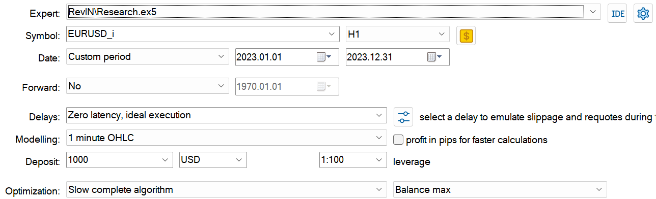
We train and test models using historical data for EURUSD, H1.
Time does not stand still. With the time, our historical database grows. So, when preparing this article, I decided to extend the historical interval of the training dataset to include the entire year 2023. Data for January 2024 will be used to test the trained models.
To create the primary training dataset, I used the Real-ORL framework. You can find its detailed description at this link. I downloaded trade data from 20 real signals. Then I ran the EA "...\Experts\RevIN\ResearchRealORL.mq5" in the Full Optimization mode.


As a result, I got 20 trajectories. Not all of them are profitable.

In this step, we first start training the Encoder. Once the Encoder training is completed, we execute the primary training for the Actor and Critic. It is primarily because 20 trajectories are too few to obtain the optimal policy of the Actor.
In the next step we expand our training dataset. For this, in slow full optimization mode, we run the EA "...\Experts\RevIN\Research.mq5". It tests the current Actor policy on real historical data within the training period and adds passes to our training dataset.

At this stage, you shouldn't expect any outstanding results. A negative result is also a result. This also serves as a good experience for further model training experiments. Moreover, such iterations assist in understanding the environment in the area of action of the Actor's current policy.
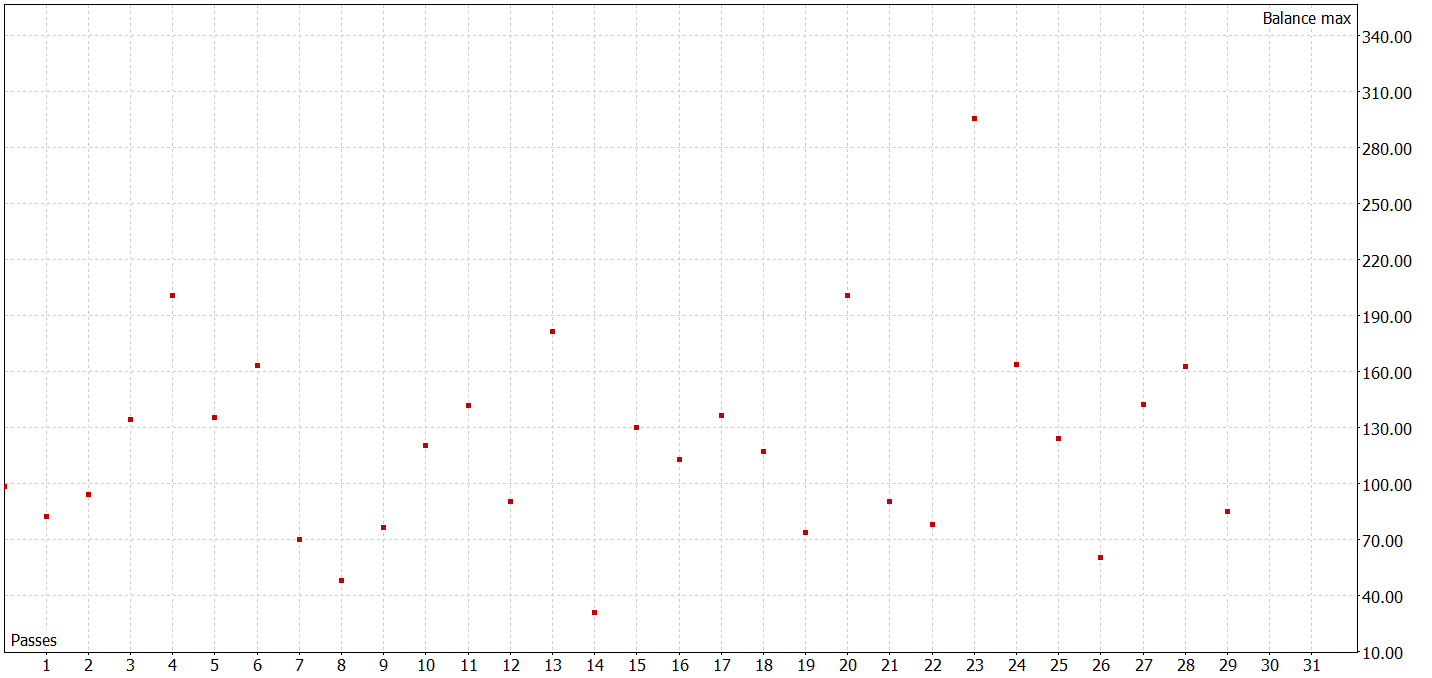
After several Actor policy training iterations and collecting additional data into the training dataset, I managed to train a model capable of generating profit on both the training and testing data sets.


During the testing period, the EA made 424 transactions, 210 of which were closed with a profit. This is 49.53%. However, since the largest and average profitable trades exceed unprofitable ones, the testing period ended up with a profit. The maximum balance and equity drawdown showed close results (9.14% and 10.36%, respectively). The profit factor for the testing period was 1.25. The Sharpe ratio reached 3.38.
Conclusion
In this article, we got acquainted with the RevIN method which represents an important step in the development of normalization and denormalization techniques. It is especially relevant for deep learning models in the context of time series forecasting. It allows us to save and retrieve statistical information about time series, which is critical for accurate forecasting. RevIN demonstrates robustness to changes in data dynamics over time. This makes it an effective tool for dealing with the problem of distribution shift in timeseries.
One of the important advantages of RevIN is its flexibility and applicability to various deep learning models. It can be easily implemented into various neural network architectures and even applied to multiple layers, providing stable prediction quality.
In the practical part of the article, we implemented the proposed approaches using MQL5. We trained models on real historical data and tested them using new data, not included in the training dataset.
The testing results showed the ability of the trained models to generalize the training data and generate profits both on historical training set and beyond.
However, it should be remembered that all programs presented in the article are of a demonstration nature and are designed only to test the proposed approaches.
References
Programs used in the article
| # | Name | Type | Description |
|---|---|---|---|
| 1 | Research.mq5 | EA | Example collection EA |
| 2 | ResearchRealORL.mq5 | EA | EA for collecting examples using the Real-ORL method |
| 3 | Study.mq5 | EA | Model training EA |
| 4 | StudyEncoder.mq5 | EA | Encode training EA |
| 5 | Test.mq5 | EA | Model testing EA |
| 6 | Trajectory.mqh | Class library | System state description structure |
| 7 | NeuroNet.mqh | Class library | A library of classes for creating a neural network |
| 8 | NeuroNet.cl | Code Base | OpenCL program code library |
Translated from Russian by MetaQuotes Ltd.
Original article: https://www.mql5.com/ru/articles/14673
Warning: All rights to these materials are reserved by MetaQuotes Ltd. Copying or reprinting of these materials in whole or in part is prohibited.
This article was written by a user of the site and reflects their personal views. MetaQuotes Ltd is not responsible for the accuracy of the information presented, nor for any consequences resulting from the use of the solutions, strategies or recommendations described.

 Creating an MQL5-Telegram Integrated Expert Advisor (Part 4): Modularizing Code Functions for Enhanced Reusability
- Free trading apps
- Over 8,000 signals for copying
- Economic news for exploring financial markets
You agree to website policy and terms of use
Neural Networks Made Easy (Part 84): Reversible Normalisation (RevIN) has been published:
Author by: Dmitriy Gizlyk
You can also simply drag and drop the image into the text or paste it using Ctrl+V
I am running the code in Neural networks made easy (Part 67): Using past experience to solve new tasks
I have the same problem regarding the following thing.
2024.04.21 18:00:01.131 Core 4 pass 0 tested with error "OnInit returned non-zero code 1" in 0:00:00.152
Looks like it is related to 'FileIsExist' command.
But, I can't resolve this issue.
Do you know how to resolve it?