
Archery Algorithm (AA)
Contents
Introduction
When tasks are becoming increasingly complex and resources are becoming increasingly scarce, optimization is becoming not only a necessity, but also a real algorithmic art in the modern world. How to find the best solution among many possible ones? How to minimize costs, increase efficiency and achieve maximum profit? These questions concern specialists in a wide range of fields – from economics to engineering, from social systems to ecology. Before solving an optimization problem, it is important to properly model the problem by identifying key variables and mathematical relationships that will adequately reproduce reality. Optimization is widely used in finance and trading, helping not only to develop new investment strategies, but also to improve existing ones. However, despite the universality of approaches, optimization methods can be conditionally divided into two categories: deterministic and stochastic.
Deterministic methods such as gradient descent offer rigorous and predictable solutions by using mathematical derivatives to find the optimum, allowing them to effectively model different scenarios, however, as soon as problems become nonlinear or multivariate, their effectiveness can decrease dramatically. In such cases, stochastic methods come to the rescue, which, relying on random processes, are able to find acceptable solutions in complex conditions, which makes them especially useful in volatile markets.Combinations of deterministic and stochastic methods play a key role in modern approaches to optimization. By combining these two approaches, analysts can create more flexible and adaptive models that can account for both stable and changing conditions. This allows not only to improve the quality of forecasts, but also to minimize risks, which is critical for successful investment management.
In this article I will present a new approach to solving optimization problems - the Archery Algorithm (AA). The algorithm was developed by Fatemeh Ahmadi Zeidabadi and colleagues and was published in February 2022. This method, inspired by archery, generates quasi-optimal solutions by updating the position of population members in the search space based on a randomly selected element. We will test the efficiency of AA on standard objective functions and compare the obtained results with algorithms already known to us. By diving into the details, we will reveal how this innovative approach can change the way we think about optimization and open up new horizons for solving complex problems.
Implementation of the algorithm
The Archery Algorithm (AA) is a completely new stochastic optimization method designed to find optimal solutions to optimization problems and inspired by the behavior of an archer aiming at a target. AA simulates the process of shooting arrows at a target. Each member of the population represents a potential solution to the optimization problem, and their positions in the search space are updated based on the performance of a randomly selected "target" member, similar to how archers adjust their aim depending on where they want to hit.
The population is represented as a matrix, where each row corresponds to a member (solution) and each column corresponds to a dimension of the problem. This allows for a structured evaluation and update of decisions based on their objective function values. The performance of each member is evaluated using an objective function that quantifies how good a found solution is. The results are stored in a vector, which allows the algorithm to compare the efficiency of different solutions.
The target is divided into sections with their width corresponding to the productivity of the population members. A probability function is calculated to determine the probability of each member being selected based on its objective function value, with more efficient archers having a higher probability of being selected. A member of the population is randomly selected based on the cumulative probability, simulating an archer's target selection. This choice affects how other members' positions are updated. The algorithm updates the position of each archer in the search space using certain equations. The update depends on whether the selected archer has a better or worse objective function value than the current one. This process involves randomness to explore the search space. AA works iteratively, updating the population until a stop condition (maximum number of iterations) is reached. During this process, the algorithm keeps track of the best solution found.
The original version of the AA algorithm presented above describes the matrix as a population and the vectors as members of the population. However, the text does not indicate specific operations that are typical for working with matrices. In fact, the algorithm includes standard actions with search agents, as in most of the previously discussed algorithms.
It is also worth noting that the phrase "the target is divided into sections with their width corresponding to the productivity of the population members" implies the use of a roulette method for selection. In this case, the probability of choosing a sector is proportional to its width.
In this way, complex formulations describing many concepts can be explained in much more simple manner simplifying the idea implementation.
So, the archery algorithm is a population-based optimization method that uses the principles of target shooting to guide the search for optimal solutions. It combines elements of randomness with normal distribution to explore and exploit the search space. Key components of the algorithm:
1. Population of agents (archers)
2. Vector of probabilities and cumulative probabilities
3. Inheritance mechanism (not present in the original version)
4. Position update mechanism
5. Training intensity parameter (I)
First, let's present the pseudocode of the algorithm:
Initialization:
Create a population of popSize agents
For each agent:
Initialize a random position within the search range
Initialize previous position and fitness
Main loop:
Until the stop condition is reached:
For each i agent in the population:
Calculate the vector of probabilities P and cumulative probabilities C
For each c coordinate:
Select k archer using cumulative probability
If (random_number < inheritance_probability):
new_position [c] = k_archer_position [c]
Otherwise:
I = rounding (1 + random_number_from_0_to_1) // Training intensity parameter
random_gaussian = generate_gaussian_number (mean = 0, min =-1, max = 1)
If (k_archer_fitness > i_agent_fitness):
new_position [c] = previous_position [c] + random_gaussian * (k_archer_position [c] - I * previous_position [c])
Otherwise:
new_position [c] = previous_position [c] + random_gaussian * (previous_position [c] - I * k_archer_position [c])
Limit new_position [c] within the search range
Update i agent position
Evaluate the fitness of all agents
Update the best global solution
For each agent:
If the new fitness is better than the previous one:
Update the previous position and fitness
Return the best solution found
Implementation features in the code:
1. The algorithm uses a probabilistic approach to select archers to learn from.
2. The inheritance mechanism allows agents to directly copy the positions of successful archers with some probability.
3. When updating positions, a Gaussian distribution is used to introduce randomness into the archers' learning process.
4. The algorithm stores the previous best positions of the agents, which allows it to have some "memory" of good decisions.
5. The implementation will include a mechanism to limit new positions within the allowed search range.
6. The training intensity parameter (I) described by the authors will be used to regulate the degree of influence of the current position on the new one.
The I parameter (training intensity) is a random variable that can take the value 1 or 2. It is defined as follows: I = rounding to the nearest integer (1 + randomly generated number from 0 to 1). This means that I will be equal to 1 with probability 0.5 and 2 with the same probability. The role of the I parameter in the algorithm:
1. When I = 1, the algorithm makes smaller position adjustments.
2. When I = 2, the algorithm can make more drastic changes in a position.
Let's move on to the algorithm code. Describe the "archer" structure - S_AA_Agent. It represents an agent in an optimization algorithm with a set of coordinates in the solution space and contains information about its efficiency in terms of the fitness function.
- cPrev [] - the array stores the previous agent coordinates.
- fPrev - the variable stores the previous value of the agent fitness.
The Init method allows us to prepare the agent for work by setting initial values for its coordinates and fitness. Next, the value is set to fPrev to the minimum possible value for the "double" type, because the fitness has not yet been calculated.
//——————————————————————————————————————————————————————————————————————————————
struct S_AA_Agent
{
    double cPrev []; // previous coordinates
    double fPrev;    // previous fitness

    void Init (int coords)
    {
      ArrayResize (cPrev, coords);
      fPrev = -DBL_MAX;
    }
};
//——————————————————————————————————————————————————————————————————————————————
Let's take a look at the C_AO_AAm class, which implements the algorithm itself and is inherited from the C_AO class.
- popSize - population size.
- inhProbab - probability of inheriting a feature from another archer.
Then the params array is initialized by the size of 2, where the algorithm parameters are stored: population size and inheritance probability.
- SetParams - method sets the parameters based on the values stored in the params array. It extracts values for popSize and inhProbab converting them to the appropriate types.
- Init - the method initializes the algorithm by accepting the minimum and maximum search boundaries, the search step, and the number of epochs.
- Moving and Revision - the methods are responsible for the logic of moving agents in the solution space and their revision (updating).
S_AA_Agent agent [] - array of agents that will be used to perform optimization.
The C_AO_AAm class implements the optimization algorithm, while SetParams, Init, Moving and Revision manage the configuration and behavior of the algorithm during its operation.
//——————————————————————————————————————————————————————————————————————————————
class C_AO_AAm : public C_AO
{
  public: //--------------------------------------------------------------------
  ~C_AO_AAm () { }
  C_AO_AAm ()
  {
    ao_name = "AAm";
    ao_desc = "Archery Algorithm M";
    ao_link = "https://www.mql5.com/en/articles/15782";

    popSize   = 50;    // population size
    inhProbab = 0.3;

    ArrayResize (params, 2);

    params [0].name = "popSize";   params [0].val = popSize;
    params [1].name = "inhProbab"; params [1].val = inhProbab;
  }

  void SetParams ()
  {
    popSize   = (int)params [0].val;
    inhProbab = params      [1].val;
  }

  bool Init (const double &rangeMinP  [], // minimum search range
             const double &rangeMaxP  [], // maximum search range
             const double &rangeStepP [], // step search
             const int     epochsP = 0);  // number of epochs

  void Moving ();
  void Revision ();

  //----------------------------------------------------------------------------
  double  inhProbab; //probability of inheritance

  S_AA_Agent agent [];

  private: //-------------------------------------------------------------------
};
//——————————————————————————————————————————————————————————————————————————————
The Init method in the C_AO_AAm class is responsible for initializing the optimization algorithm. It takes four parameters: arrays for the minimum and maximum search bounds, the search step, and the number of epochs that are equal to zero by default.
- If the standard initialization is successful, the method resizes the agent, so that it corresponds to the specified popSize population size. This allows us to create the required number of agents to be used in the algorithm.
- In the for loop, each agent from the array is initialized using the Init method, which specifies the initial coordinates for each agent.
At the end, the method returns true, indicating successful completion of the algorithm initialization. Thus, the Init method ensures that the algorithm is prepared for operation by setting up the necessary parameters and creating agents that will participate in the optimization.
//——————————————————————————————————————————————————————————————————————————————
bool C_AO_AAm::Init (const double &rangeMinP  [],
                     const double &rangeMaxP  [],
                     const double &rangeStepP [],
                     const int     epochsP = 0)
{
  if (!StandardInit (rangeMinP, rangeMaxP, rangeStepP)) return false;

  //----------------------------------------------------------------------------
  ArrayResize (agent, popSize);
  for (int i = 0; i < popSize; i++) agent [i].Init (coords);

  return true;
}
//——————————————————————————————————————————————————————————————————————————————
The Moving method in the C_AO_AAm class is responsible for moving agents in the solution space based on their current positions and the values of the function they are optimizing. Let's break it down into parts:
- If the method is called for the first time (revision is equal to false), then a random value is initialized within the specified boundaries of rangeMin and rangeMax for each agent and each coordinate.
- Then, this value is adjusted using the SeInDiSp method, which ensures that the value matches the specified step.
After that, the revision flag is set to true and the method completes its work.
- Two arrays are created next: P for probabilities and C for cumulative probabilities.
- The F_worst worst value of the function is found to normalize the fitness function values for agents.
- The probabilities for each agent are then calculated and normalized so that they sum to 1.
- C cumulative probabilities are calculated based on P probabilities.
- For each agent and each coordinate, a partner archer (an agent) is selected based on cumulative probability.
- If the random value is less than the specified inhProbab inheritance probability, the agent accepts the coordinate of the selected agent (ensuring the inheritance of features with a given probability).
- Otherwise, the agent updates its position based on an equation that takes into account the current position, the random value, and the position of the partner shooter.
- Finally, the new coordinate value is also adjusted using the SeInDiSp method.
The Moving method implements the movement of agents in the solution space taking into account their current positions and function values and uses probabilistic methods to select directions of movement and update positions.
//——————————————————————————————————————————————————————————————————————————————
void C_AO_AAm::Moving ()
{
  //----------------------------------------------------------------------------
  if (!revision)
  {
    for (int i = 0; i < popSize; i++)
    {
      for (int c = 0; c < coords; c++)
      {
        a [i].c [c] = u.RNDfromCI (rangeMin [c], rangeMax [c]);
        a [i].c [c] = u.SeInDiSp (a [i].c [c], rangeMin [c], rangeMax [c], rangeStep [c]);
      }
    }
    revision = true;
    return;
  }

  //-------------------------------------------------------------------------
  // Calculate probability vector P and cumulative probability C
  double P [], C [];
  ArrayResize (P, popSize);
  ArrayResize (C, popSize);
  double F_worst = DBL_MAX;
  double sum = 0;

  for (int i = 0; i < popSize; i++)
  {
    if (a [i].f < F_worst) F_worst = a [i].f;
  }

  for (int i = 0; i < popSize; i++)
  {
    P [i] =  a [i].f - F_worst;
    sum += P [i];
  }

  for (int i = 0; i < popSize; i++)
  {
    P [i] /= sum;
    C [i] = (i == 0) ? P [i] : C [i - 1] + P [i];
  }

  double x;

  for (int i = 0; i < popSize; i++)
  {
    for (int c = 0; c < coords; c++)
    {
      // Select archer (k) using cumulative probability
      int k = 0;
      double r = u.RNDprobab ();
      while (k < popSize - 1 && C [k] < r) k++;

      if (u.RNDbool () < inhProbab)
      {
        x = a [k].c [c];
      }
      else
      {
        // Update position using Eq. (5) and (6)
        double I   = MathRound (1 + u.RNDprobab ());
        double rnd = u.GaussDistribution (0, -1, 1, 8);

        if (a [k].f > a [i].f)
        {
          x = agent [i].cPrev [c] + rnd * (a [k].c [c] - I * agent [i].cPrev [c]);
        }
        else
        {
          x = agent [i].cPrev [c] + rnd * (agent [i].cPrev [c] - I * a [k].c [c]);
        }
      }

      a [i].c [c] = u.SeInDiSp (x, rangeMin [c], rangeMax [c], rangeStep [c]);
    }
  }
}
//——————————————————————————————————————————————————————————————————————————————
The Revision method in the C_AO_AAm class is responsible for updating information about the best agents in the population. The method does the following:
- The ind variable is initialized with the value of -1. It will be used to store the index of the agent with the best function value.
- The for loop iterates through all agents in the popSize population and if the value of the a [i].f current agent function exceeds the current best value of the fB function:
- fB is updated to the new better value of a [i].f.
- the index of this agent is stored in the ind variable.
- If the value of the a [i].f current agent function exceeds its previous agent [i].fPrev fitness function value:
- the previous value of fPrev for the agent is updated.
- the current coordinates of the agent are copied to the cPrev array using ArrayCopy.
The Revision method serves to update information about the best global solution, as well as to update the best positions of agents.
//——————————————————————————————————————————————————————————————————————————————
void C_AO_AAm::Revision ()
{
  //----------------------------------------------------------------------------
  int ind = -1;

  for (int i = 0; i < popSize; i++)
  {
    if (a [i].f > fB)
    {
      fB = a [i].f;
      ind = i;
    }
  }

  if (ind != -1) ArrayCopy (cB, a [ind].c, 0, 0, WHOLE_ARRAY);

  //----------------------------------------------------------------------------
  for (int i = 0; i < popSize; i++)
  {
    if (a [i].f > agent [i].fPrev)
    {
      agent [i].fPrev = a [i].f;
      ArrayCopy (agent [i].cPrev, a [i].c, 0, 0, WHOLE_ARRAY);
    }
  }
}
//——————————————————————————————————————————————————————————————————————————————
Test results
I have slightly modified the algorithm. The original algorithm does not provide for direct exchange of information between archers. The exchange occurs indirectly through the interaction of coordinates via the normal distribution, so I thought it was necessary to add the exchange of such information. For this purpose, I have added the additional inhProbab algorithm responsible for implementing such an exchange with a given probability.
if (u.RNDbool () < inhProbab)
{
  x = a [k].c [c];
}
The results presented below correspond to the original version of the algorithm as intended by the authors.
AA|Archery Algorithm|50.0|
=============================
5 Hilly's; Func runs: 10000; result: 0.6699547926310098
25 Hilly's; Func runs: 10000; result: 0.37356238340164605
500 Hilly's; Func runs: 10000; result: 0.257542163368952
=============================
5 Forest's; Func runs: 10000; result: 0.38166669771790607
25 Forest's; Func runs: 10000; result: 0.199300365268835
500 Forest's; Func runs: 10000; result: 0.15337954055780398
=============================
5 Megacity's; Func runs: 10000; result: 0.4076923076923077
25 Megacity's; Func runs: 10000; result: 0.17907692307692308
500 Megacity's; Func runs: 10000; result: 0.10004615384615476
=============================
All score: 2.72222 (30.25%)
The algorithm scores 30.25% in the test, but with my modification the algorithm improved its performance by more than 13%. Below are the results of the modified version:
AAm|Archery Algorithm M|50.0|0.3|
=============================
5 Hilly's; Func runs: 10000; result: 0.9353194829441194
25 Hilly's; Func runs: 10000; result: 0.6798262991897616
500 Hilly's; Func runs: 10000; result: 0.2596620178276653
=============================
5 Forest's; Func runs: 10000; result: 0.5735062785421186
25 Forest's; Func runs: 10000; result: 0.22007188891556378
500 Forest's; Func runs: 10000; result: 0.1486980566819649
=============================
5 Megacity's; Func runs: 10000; result: 0.6307692307692309
25 Megacity's; Func runs: 10000; result: 0.344
500 Megacity's; Func runs: 10000; result: 0.10193846153846249
=============================
All score: 3.89379 (43.26%)
So, I have selected the algorithm with modification and added it to the rating table. Below we can see the algorithm visualization. I think it is quite good. There is, of course, a spread of results, however, it is not critical and occurs only for functions with a small number of coordinates.
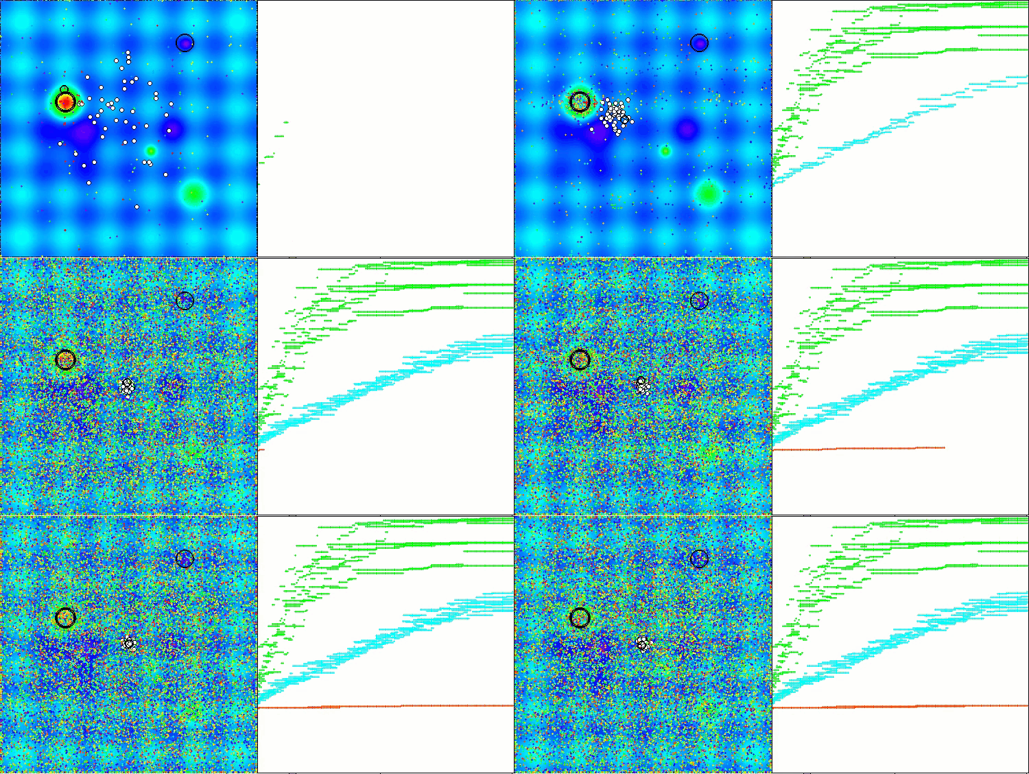
AAm on the Hilly test function
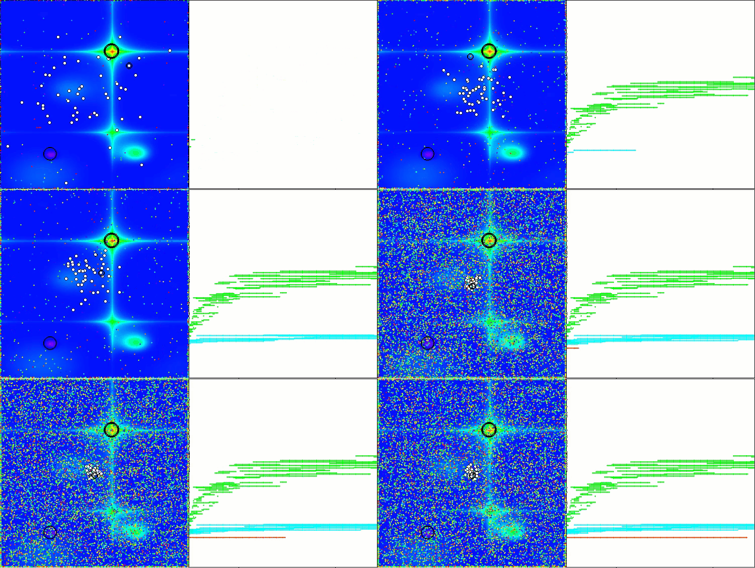
AAm on the Forest test function
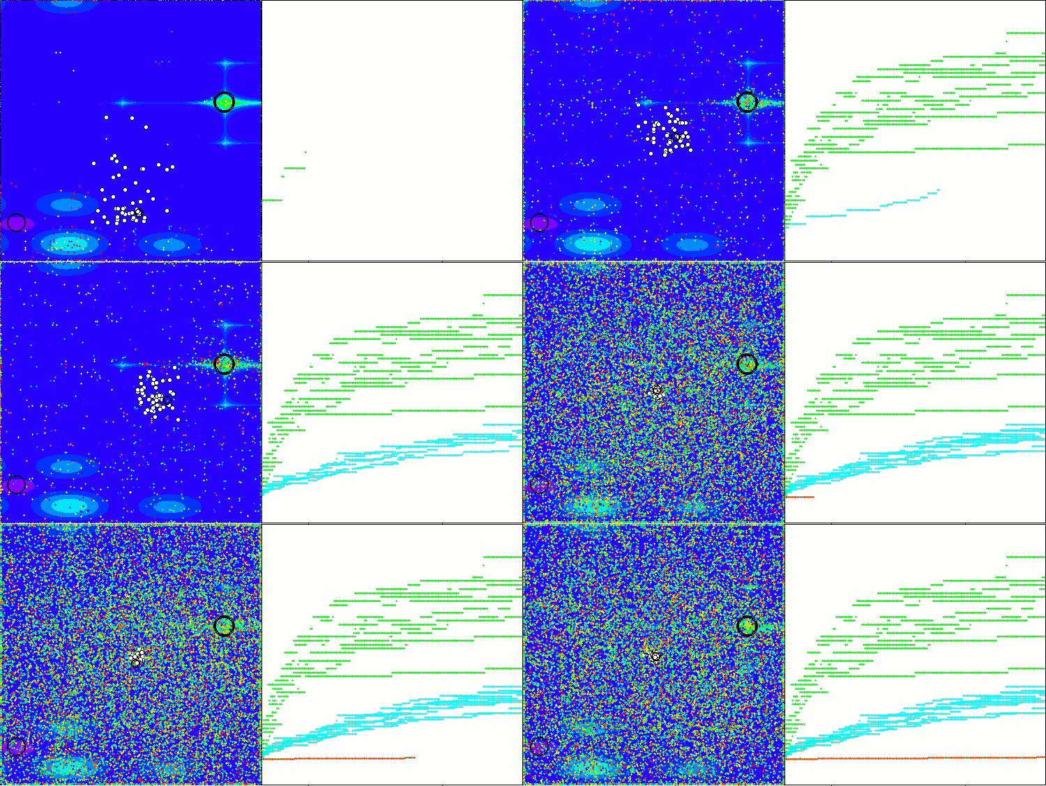
AAm on the Megacity test function
According to the operation results, the modified version of the algorithm occupies 26 th place.
| # | AO | Description | Hilly | Hilly final | Forest | Forest final | Megacity (discrete) | Megacity final | Final result | % of MAX | ||||||
| 10 p (5 F) | 50 p (25 F) | 1000 p (500 F) | 10 p (5 F) | 50 p (25 F) | 1000 p (500 F) | 10 p (5 F) | 50 p (25 F) | 1000 p (500 F) | ||||||||
| 1 | ANS | across neighbourhood search | 0.94948 | 0.84776 | 0.43857 | 2.23581 | 1.00000 | 0.92334 | 0.39988 | 2.32323 | 0.70923 | 0.63477 | 0.23091 | 1.57491 | 6.134 | 68.15 |
| 2 | CLA | code lock algorithm | 0.95345 | 0.87107 | 0.37590 | 2.20042 | 0.98942 | 0.91709 | 0.31642 | 2.22294 | 0.79692 | 0.69385 | 0.19303 | 1.68380 | 6.107 | 67.86 |
| 3 | AMOm | animal migration ptimization M | 0.90358 | 0.84317 | 0.46284 | 2.20959 | 0.99001 | 0.92436 | 0.46598 | 2.38034 | 0.56769 | 0.59132 | 0.23773 | 1.39675 | 5.987 | 66.52 |
| 4 | (P+O)ES | (P+O) evolution strategies | 0.92256 | 0.88101 | 0.40021 | 2.20379 | 0.97750 | 0.87490 | 0.31945 | 2.17185 | 0.67385 | 0.62985 | 0.18634 | 1.49003 | 5.866 | 65.17 |
| 5 | CTA | comet tail algorithm | 0.95346 | 0.86319 | 0.27770 | 2.09435 | 0.99794 | 0.85740 | 0.33949 | 2.19484 | 0.88769 | 0.56431 | 0.10512 | 1.55712 | 5.846 | 64.96 |
| 6 | SDSm | stochastic diffusion search M | 0.93066 | 0.85445 | 0.39476 | 2.17988 | 0.99983 | 0.89244 | 0.19619 | 2.08846 | 0.72333 | 0.61100 | 0.10670 | 1.44103 | 5.709 | 63.44 |
| 7 | ESG | evolution of social groups | 0.99906 | 0.79654 | 0.35056 | 2.14616 | 1.00000 | 0.82863 | 0.13102 | 1.95965 | 0.82333 | 0.55300 | 0.04725 | 1.42358 | 5.529 | 61.44 |
| 8 | SIA | simulated isotropic annealing | 0.95784 | 0.84264 | 0.41465 | 2.21513 | 0.98239 | 0.79586 | 0.20507 | 1.98332 | 0.68667 | 0.49300 | 0.09053 | 1.27020 | 5.469 | 60.76 |
| 9 | ACS | artificial cooperative search | 0.75547 | 0.74744 | 0.30407 | 1.80698 | 1.00000 | 0.88861 | 0.22413 | 2.11274 | 0.69077 | 0.48185 | 0.13322 | 1.30583 | 5.226 | 58.06 |
| 10 | ASO | anarchy society optimization | 0.84872 | 0.74646 | 0.31465 | 1.90983 | 0.96148 | 0.79150 | 0.23803 | 1.99101 | 0.57077 | 0.54062 | 0.16614 | 1.27752 | 5.178 | 57.54 |
| 11 | TSEA | turtle shell evolution algorithm | 0.96798 | 0.64480 | 0.29672 | 1.90949 | 0.99449 | 0.61981 | 0.22708 | 1.84139 | 0.69077 | 0.42646 | 0.13598 | 1.25322 | 5.004 | 55.60 |
| 12 | DE | differential evolution | 0.95044 | 0.61674 | 0.30308 | 1.87026 | 0.95317 | 0.78896 | 0.16652 | 1.90865 | 0.78667 | 0.36033 | 0.02953 | 1.17653 | 4.955 | 55.06 |
| 13 | CRO | chemical reaction optimization | 0.94629 | 0.66112 | 0.29853 | 1.90593 | 0.87906 | 0.58422 | 0.21146 | 1.67473 | 0.75846 | 0.42646 | 0.12686 | 1.31178 | 4.892 | 54.36 |
| 14 | BSA | bird swarm algorithm | 0.89306 | 0.64900 | 0.26250 | 1.80455 | 0.92420 | 0.71121 | 0.24939 | 1.88479 | 0.69385 | 0.32615 | 0.10012 | 1.12012 | 4.809 | 53.44 |
| 15 | HS | harmony search | 0.86509 | 0.68782 | 0.32527 | 1.87818 | 0.99999 | 0.68002 | 0.09590 | 1.77592 | 0.62000 | 0.42267 | 0.05458 | 1.09725 | 4.751 | 52.79 |
| 16 | SSG | saplings sowing and growing | 0.77839 | 0.64925 | 0.39543 | 1.82308 | 0.85973 | 0.62467 | 0.17429 | 1.65869 | 0.64667 | 0.44133 | 0.10598 | 1.19398 | 4.676 | 51.95 |
| 17 | BCOm | bacterial chemotaxis optimization M | 0.75953 | 0.62268 | 0.31483 | 1.69704 | 0.89378 | 0.61339 | 0.22542 | 1.73259 | 0.65385 | 0.42092 | 0.14435 | 1.21912 | 4.649 | 51.65 |
| 18 | (PO)ES | (PO) evolution strategies | 0.79025 | 0.62647 | 0.42935 | 1.84606 | 0.87616 | 0.60943 | 0.19591 | 1.68151 | 0.59000 | 0.37933 | 0.11322 | 1.08255 | 4.610 | 51.22 |
| 19 | TSm | tabu search M | 0.87795 | 0.61431 | 0.29104 | 1.78330 | 0.92885 | 0.51844 | 0.19054 | 1.63783 | 0.61077 | 0.38215 | 0.12157 | 1.11449 | 4.536 | 50.40 |
| 20 | BSO | brain storm optimization | 0.93736 | 0.57616 | 0.29688 | 1.81041 | 0.93131 | 0.55866 | 0.23537 | 1.72534 | 0.55231 | 0.29077 | 0.11914 | 0.96222 | 4.498 | 49.98 |
| 21 | WOAm | wale optimization algorithm M | 0.84521 | 0.56298 | 0.26263 | 1.67081 | 0.93100 | 0.52278 | 0.16365 | 1.61743 | 0.66308 | 0.41138 | 0.11357 | 1.18803 | 4.476 | 49.74 |
| 22 | AEFA | artificial electric field algorithm | 0.87700 | 0.61753 | 0.25235 | 1.74688 | 0.92729 | 0.72698 | 0.18064 | 1.83490 | 0.66615 | 0.11631 | 0.09508 | 0.87754 | 4.459 | 49.55 |
| 23 | ACOm | ant colony optimization M | 0.88190 | 0.66127 | 0.30377 | 1.84693 | 0.85873 | 0.58680 | 0.15051 | 1.59604 | 0.59667 | 0.37333 | 0.02472 | 0.99472 | 4.438 | 49.31 |
| 24 | BFO-GA | bacterial foraging optimization - ga | 0.89150 | 0.55111 | 0.31529 | 1.75790 | 0.96982 | 0.39612 | 0.06305 | 1.42899 | 0.72667 | 0.27500 | 0.03525 | 1.03692 | 4.224 | 46.93 |
| 25 | ABHA | artificial bee hive algorithm | 0.84131 | 0.54227 | 0.26304 | 1.64663 | 0.87858 | 0.47779 | 0.17181 | 1.52818 | 0.50923 | 0.33877 | 0.10397 | 0.95197 | 4.127 | 45.85 |
| 26 | AAm | archery algorithm M | 0.93532 | 0.67983 | 0.25966 | 1.87481 | 0.57351 | 0.22007 | 0.14870 | 0.94228 | 0.63077 | 0.34400 | 0.10194 | 1.07671 | 3.894 | 43.26 |
| 27 | ASBO | adaptive social behavior optimization | 0.76331 | 0.49253 | 0.32619 | 1.58202 | 0.79546 | 0.40035 | 0.26097 | 1.45677 | 0.26462 | 0.17169 | 0.18200 | 0.61831 | 3.657 | 40.63 |
| 28 | MEC | mind evolutionary computation | 0.69533 | 0.53376 | 0.32661 | 1.55569 | 0.72464 | 0.33036 | 0.07198 | 1.12698 | 0.52500 | 0.22000 | 0.04198 | 0.78698 | 3.470 | 38.55 |
| 29 | IWO | invasive weed optimization | 0.72679 | 0.52256 | 0.33123 | 1.58058 | 0.70756 | 0.33955 | 0.07484 | 1.12196 | 0.42333 | 0.23067 | 0.04617 | 0.70017 | 3.403 | 37.81 |
| 30 | Micro-AIS | micro artificial immune system | 0.79547 | 0.51922 | 0.30861 | 1.62330 | 0.72956 | 0.36879 | 0.09398 | 1.19233 | 0.37667 | 0.15867 | 0.02802 | 0.56335 | 3.379 | 37.54 |
| 31 | COAm | cuckoo optimization algorithm M | 0.75820 | 0.48652 | 0.31369 | 1.55841 | 0.74054 | 0.28051 | 0.05599 | 1.07704 | 0.50500 | 0.17467 | 0.03380 | 0.71347 | 3.349 | 37.21 |
| 32 | SDOm | spiral dynamics optimization M | 0.74601 | 0.44623 | 0.29687 | 1.48912 | 0.70204 | 0.34678 | 0.10944 | 1.15826 | 0.42833 | 0.16767 | 0.03663 | 0.63263 | 3.280 | 36.44 |
| 33 | NMm | Nelder-Mead method M | 0.73807 | 0.50598 | 0.31342 | 1.55747 | 0.63674 | 0.28302 | 0.08221 | 1.00197 | 0.44667 | 0.18667 | 0.04028 | 0.67362 | 3.233 | 35.92 |
| 34 | FAm | firefly algorithm M | 0.58634 | 0.47228 | 0.32276 | 1.38138 | 0.68467 | 0.37439 | 0.10908 | 1.16814 | 0.28667 | 0.16467 | 0.04722 | 0.49855 | 3.048 | 33.87 |
| 35 | GSA | gravitational search algorithm | 0.64757 | 0.49197 | 0.30062 | 1.44016 | 0.53962 | 0.36353 | 0.09945 | 1.00260 | 0.32667 | 0.12200 | 0.01917 | 0.46783 | 2.911 | 32.34 |
| 36 | BFO | bacterial foraging optimization | 0.61171 | 0.43270 | 0.31318 | 1.35759 | 0.54410 | 0.21511 | 0.05676 | 0.81597 | 0.42167 | 0.13800 | 0.03195 | 0.59162 | 2.765 | 30.72 |
| 37 | ABC | artificial bee colony | 0.63377 | 0.42402 | 0.30892 | 1.36671 | 0.55103 | 0.21874 | 0.05623 | 0.82600 | 0.34000 | 0.14200 | 0.03102 | 0.51302 | 2.706 | 30.06 |
| 38 | BA | bat algorithm | 0.59761 | 0.45911 | 0.35242 | 1.40915 | 0.40321 | 0.19313 | 0.07175 | 0.66810 | 0.21000 | 0.10100 | 0.03517 | 0.34617 | 2.423 | 26.93 |
| 39 | AAA | algae adaptive algorithm | 0.50007 | 0.32040 | 0.25525 | 1.07572 | 0.37021 | 0.22284 | 0.16785 | 0.76089 | 0.27846 | 0.14800 | 0.09755 | 0.52402 | 2.361 | 26.23 |
| 40 | SA | simulated annealing | 0.55787 | 0.42177 | 0.31549 | 1.29513 | 0.34998 | 0.15259 | 0.05023 | 0.55280 | 0.31167 | 0.10033 | 0.02883 | 0.44083 | 2.289 | 25.43 |
| 41 | IWDm | intelligent water drops M | 0.54501 | 0.37897 | 0.30124 | 1.22522 | 0.46104 | 0.14704 | 0.04369 | 0.65177 | 0.25833 | 0.09700 | 0.02308 | 0.37842 | 2.255 | 25.06 |
| 42 | PSO | particle swarm optimisation | 0.59726 | 0.36923 | 0.29928 | 1.26577 | 0.37237 | 0.16324 | 0.07010 | 0.60572 | 0.25667 | 0.08000 | 0.02157 | 0.35823 | 2.230 | 24.77 |
| 43 | Boids | boids algorithm | 0.43340 | 0.30581 | 0.25425 | 0.99346 | 0.35718 | 0.20160 | 0.15708 | 0.71586 | 0.27846 | 0.14277 | 0.09834 | 0.51957 | 2.229 | 24.77 |
| 44 | MA | monkey algorithm | 0.59107 | 0.42681 | 0.31816 | 1.33604 | 0.31138 | 0.14069 | 0.06612 | 0.51819 | 0.22833 | 0.08567 | 0.02790 | 0.34190 | 2.196 | 24.40 |
| 45 | SFL | shuffled frog-leaping | 0.53925 | 0.35816 | 0.29809 | 1.19551 | 0.37141 | 0.11427 | 0.04051 | 0.52618 | 0.27167 | 0.08667 | 0.02402 | 0.38235 | 2.104 | 23.38 |
Summary
i have presented two versions of the algorithm: the original and modified one, which includes minor changes, but provides a significant improvement in performance. This article clearly demonstrates that even minor adjustments to the logic of an algorithm can lead to significant gains in efficiency in various tasks. It also becomes clear that complex descriptions can make it difficult to understand how an algorithm works, which in turn hinders its improvement. On the contrary, complex concepts expressed in simple language open the way to more efficient solutions.
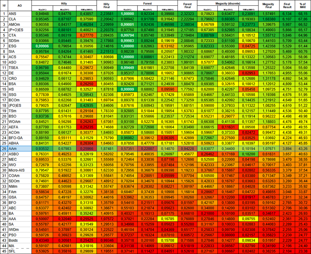
Figure 1. Color gradation of algorithms according to relevant tests Results greater than or equal to 0.99 are highlighted in white
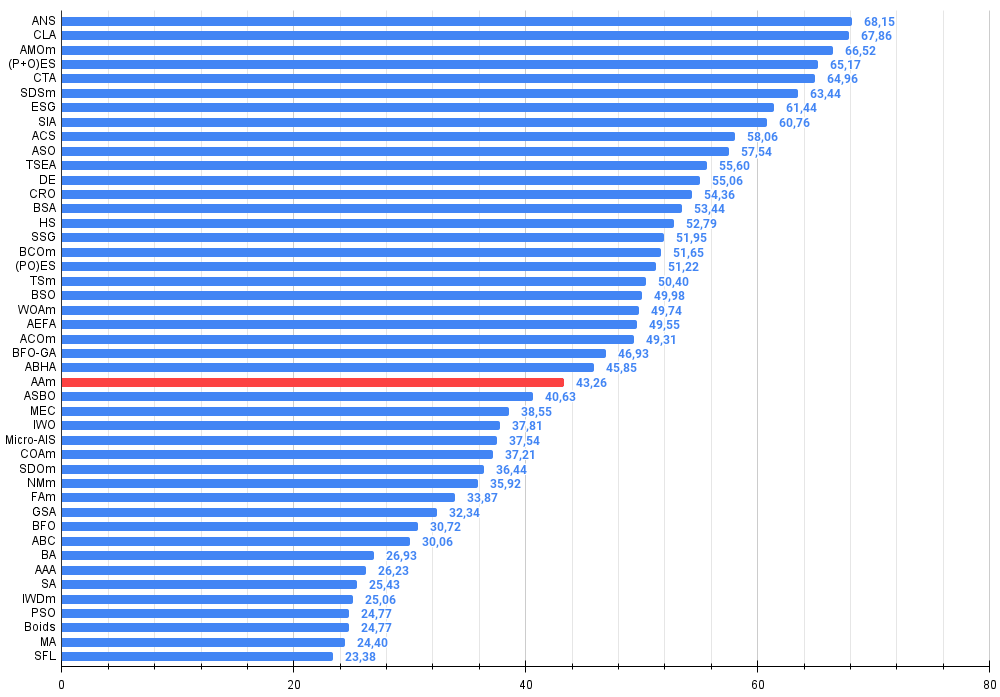
Figure 2. Histogram of algorithm testing results (scale from 0 to 100, the higher the better, where 100 is the maximum possible theoretical result, in the archive there is a script for calculating the rating table)
When the article was almost ready for publication, I had an idea that I decided to test. What if, following the logic of the authors about targets and archers using the "roulette" method for selection, we change the sizes of the targets themselves inversely proportional to the quality of the solutions found? If the solution turns out to be good, it should be refined and its surroundings explored. Otherwise, if the result is insignificant, it is necessary to expand the search area to identify new, potentially promising areas.
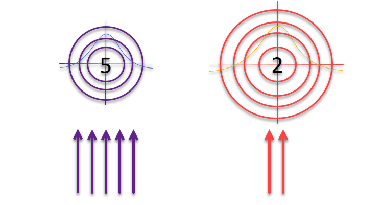
Figure 3. The number of arrows hitting the targets is directly proportional to the quality of the targets themselves, while the size of the targets is inversely proportional to their quality
Let's look at the code that uses the idea of increasing targets inversely proportional to their quality.
void C_AO_AAm::Moving ()
{
  //----------------------------------------------------------------------------
  if (!revision)
  {
    for (int i = 0; i < popSize; i++)
    {
      for (int c = 0; c < coords; c++)
      {
        a [i].c [c] = u.RNDfromCI (rangeMin [c], rangeMax [c]);
        a [i].c [c] = u.SeInDiSp (a [i].c [c], rangeMin [c], rangeMax [c], rangeStep [c]);
      }
    }
    revision = true;
    return;
  }

  //-------------------------------------------------------------------------
  // Calculate probability vector P and cumulative probability C
  double P [], C [];
  ArrayResize (P, popSize);
  ArrayResize (C, popSize);
  double F_worst = DBL_MAX; // a[ArrayMaximum(a, WHOLE_ARRAY, 0, popSize)].f;
  double sum = 0;

  for (int i = 0; i < popSize; i++)
  {
    if (a [i].f < F_worst) F_worst = a [i].f;
  }

  for (int i = 0; i < popSize; i++)
  {
    P [i] =  a [i].f - F_worst; ////F_worst - a[i].f;
    sum += P [i];
  }

  for (int i = 0; i < popSize; i++)
  {
    P [i] /= sum;
    C [i] = (i == 0) ? P [i] : C [i - 1] + P [i];
  }

  double x;

  double maxFF = fB;
  double minFF = DBL_MAX;
  double prob1;
  double prob2;

  for (int i = 0; i < popSize; i++)
  {
    if (a [i].f < minFF) minFF = a [i].f;
  }

  for (int i = 0; i < popSize; i++)
  {
    for (int c = 0; c < coords; c++)
    {
      // Select archer (k) using cumulative probability
      int k = 0;
      double r = u.RNDprobab ();
      while (k < popSize - 1 && C [k] < r) k++;

      if (u.RNDbool () < inhProbab)
      {
        x = a [k].c [c];
      }
      else
      {

        // Update position using Eq. (5) and (6)
        //double I   = MathRound (1 + u.RNDprobab ());
        double rnd = u.GaussDistribution (0, -1, 1, 8);
        /*
        if (a [k].f > a [i].f)
        {
          x = agent [i].cPrev [c] + rnd * (a [k].c [c] - I * agent [i].cPrev [c]);
        }
        else
        {
          x = agent [i].cPrev [c] + rnd * (agent [i].cPrev [c] - I * a [k].c [c]);
        }
        */

        prob1 = u.Scale (a [i].f, minFF, maxFF, 0, 1);
        prob2 = u.Scale (a [k].f, minFF, maxFF, 0, 1);

        x = agent [i].cPrev [c] + rnd * (a [k].c [c] - agent [i].cPrev [c]) * (1 - prob1 - prob2);

      }

      a [i].c [c] = u.SeInDiSp (x, rangeMin [c], rangeMax [c], rangeStep [c]);
    }
  }
}
//—
1. The commented section in the original version used the conditional construct if-else to determine how to update the agent position. This logic has been removed and replaced with a new calculation.
2. Three new strings of code:
prob1 = u.Scale(a[i].f, minFF, maxFF, 0, 1);
prob2 = u.Scale(a[k].f, minFF, maxFF, 0, 1);

x = agent[i].cPrev[c] + rnd * (a[k].c[c] - agent[i].cPrev[c]) * (1 - prob1 - prob2);
These lines introduce a new approach to calculating the updated position:
a) Two probability values (prob1 and prob2) are calculated using the Scale function, which normalizes the fitness values of i and k agents in the range from 0 to 1 based on the minFF and maxFF minimum and maximum fitness values.
b) Then the new x position is calculated using these probabilities. It uses the i previous position of the agent [i].cPrev [c] agent, k position of the a [k].c [c] selected archer and rnd random factor.
c) Now the movement is affected by the sum of the fitness values of both agents subtracted from 1. This factor serves as a scaling factor, allowing the target to be expanded or contracted in inverse proportion to the fitness of the chosen archers. The less experienced the archers, the greater the spread of arrows, but the distribution of the probabilities of hitting the targets still follows a normal distribution.
Now let's look at the results:
AAm|Archery Algorithm M|50.0|0.3|
=============================
5 Hilly's; Func runs: 10000; result: 0.9174358826544864
25 Hilly's; Func runs: 10000; result: 0.7087620527831496
500 Hilly's; Func runs: 10000; result: 0.42160091427958263
=============================
5 Forest's; Func runs: 10000; result: 0.9252690259821034
25 Forest's; Func runs: 10000; result: 0.7580206359203926
500 Forest's; Func runs: 10000; result: 0.353277934084795
=============================
5 Megacity's; Func runs: 10000; result: 0.6738461538461538
25 Megacity's; Func runs: 10000; result: 0.552
500 Megacity's; Func runs: 10000; result: 0.23738461538461658
=============================
All score: 5.54760 (61.64%)
The algorithm performance has improved significantly. In the visualization below, we can see the confident convergence of the algorithm and the identification of significant areas of the function surface.
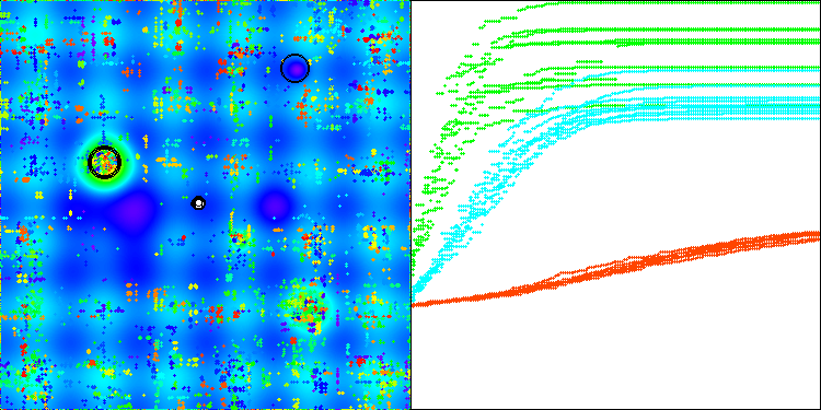
AAm on the Hilly test function
Let's conduct another small experiment. The results above are obtained by subtracting the sum of the archers' probabilities from one.
//x = agent [i].cPrev [c] + rnd * (a [k].c [c] - agent [i].cPrev [c]) * (1 - prob1 - prob2);
 x = agent [i].cPrev [c] + rnd * (a [k].c [c] - agent [i].cPrev [c]) * (2 - prob1 - prob2);
The main change is that the sum is subtracted not from one but from two. Let's see how such a simple action can affect the behavior of the algorithm:
- in the previous version, the result of this operation could be negative if the fitness of both archers was high, resulting in a "mutation" effect in the resulting coordinates of the new archer.
- in the new version the multiplier will provide a value from 0 to 2.
This change results in agents moving in a more sweeping manner and exploring the solution space more aggressively, as agents will take larger steps with each position update.
Thus, as can be seen from the printout of the algorithm's results, this change improved the convergence of the algorithm on medium-dimensional functions, but also resulted in a deterioration on high-dimensional functions (marked in yellow), although overall the algorithm scored a higher final value.
AAm|Archery Algorithm M|50.0|0.3|
=============================
5 Hilly's; Func runs: 10000; result: 0.9053229410164233
25 Hilly's; Func runs: 10000; result: 0.8259118221071665
500 Hilly's; Func runs: 10000; result: 0.2631661675236262
=============================
5 Forest's; Func runs: 10000; result: 0.9714247249319152
25 Forest's; Func runs: 10000; result: 0.9091052022399436
500 Forest's; Func runs: 10000; result: 0.2847632249786224
=============================
5 Megacity's; Func runs: 10000; result: 0.7169230769230768
25 Megacity's; Func runs: 10000; result: 0.6378461538461538
500 Megacity's; Func runs: 10000; result: 0.10473846153846252
=============================
All score: 5.61920 (62.44%)
The previous result looks more practical and will remain as the main variant of the modified version of the AAm algorithm. I will present the rating table with thermal gradation once again. AAm now occupies a worthy 7 th place. The algorithm can be characterized as very balanced (good convergence on functions of different dimensions) and can be recommended for solving various problems.
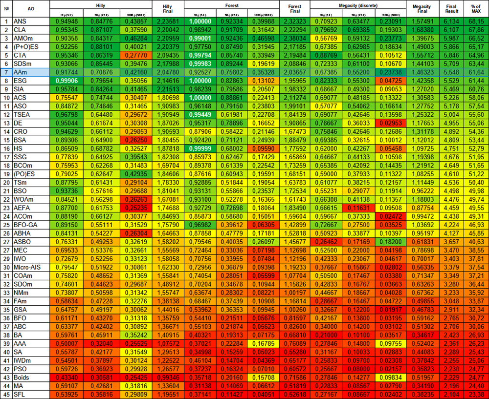
Figure 4. Color gradation of algorithms according to relevant tests Results greater than or equal to 0.99 are highlighted in white
AAm pros and cons:
Pros:
- Quite fast.
- Self-adaptive.
- Just one external parameter.
- Good convergence.
- Good scalability.
- Simple implementation (despite the complex description made by the authors).
Cons:
- Somewhat prone to getting stuck on low dimensional functions.
Further addition of new algorithms to the rating table will make it difficult to read. Therefore, I decided to limit the number of rating participants to 45 algorithms, and now the competition is held in a "knockout" format. To make it easy for readers to access all the articles in a visually appealing way, I have prepared an HTML file with a list of all the previously reviewed algorithms, sorted by their rating in a table. This file has been present in the article archive for some time now, and for those who open it for the first time, there is a little surprise in store.
The article is accompanied by an archive with the current versions of the algorithm codes. The author of the article is not responsible for the absolute accuracy in the description of canonical algorithms. Changes have been made to many of them to improve search capabilities. The conclusions and judgments presented in the articles are based on the results of the experiments.
Translated from Russian by MetaQuotes Ltd.
Original article: https://www.mql5.com/ru/articles/15782
 Neural Network in Practice: The First Neuron
 Simple solutions for handling indicators conveniently
 Advanced Memory Management and Optimization Techniques in MQL5
 Automating Trading Strategies in MQL5 (Part 13): Building a Head and Shoulders Trading Algorithm
- Free trading apps
- Over 8,000 signals for copying
- Economic news for exploring financial markets
You agree to website policy and terms of use
Thanks for your interest in my work and great question.
There are many scenarios for applying optimisation algorithms, wherever you want to get the best solution among the possible ones.
For example, you can apply it to self-optimisation of EAs as described here.
Or it can be used as part of the optimisation management of an in-house tester, as described here.