Build Self Optimizing Expert Advisors in MQL5 (Part 6): Self Adapting Trading Rules (II)

MetaTrader 5 — Examples | 28 March 2025, 16:22

2 474

In our last discussion on self adapting trading rules, linked here, we considered the problems faced by an algorithmic trader attempting to follow best practices on how to follow the RSI indicator.

We found that the standardized results aren’t always generated by the indicator, depending on several factors, such as the period, time frame and also the particular market in question.

To resolve this issue, we postulated that algorithmic traders could rather study the true range of the indicator, so they can readjust the midpoint of the indicator, to the middle of its observed range, and not its total possible range. Doing so, gives us some guarantees about the generation of trading signals, that we cannot obtain from the traditional rules of the RSI. We gained additional control over the new signal by recording an average deviation from the mid-point, and only registering signals generated by multiples of the average deviation.

We shall now advance beyond our initial attempt to build a practical solution. There are several improvements we can make over our last attempt. The integral improvement we seek is the ability to try to estimate the value of our chosen RSI levels.

In our last discussion, we simply assumed that deviations significantly larger than the average deviation could tend to be more profitable. However, we did not attempt to measure if this was true. We made no attempt to quantify the value of the new levels we are proposing and compare them against the value of the traditional levels, 70 and 30.

Additionally, our last discussion considered the case where the RSI period was fixed. This simplifying assumption made our framework easier to understand. Today, we turn our attention to the opposite end of the problem, when the practitioner is uncertain of the right period to use.

Visualizing The Problem

In case we have new readers joining us, In Fig 1 below, we have attached a screenshot of the Daily EURUSD chart with a 2 period RSI.

Fig 1

Fig 1: Visualizing our RSI the quality of signals generated by a short period.

Underneath Fig 1, we have applied a 70 period RSI to the same section of the chart in Fig 2. We can observe the RSI signal is slowly becoming a flat line centered along the 50 RSI level. What comments could we make when we compare the 2 pictures? Well, one comment worth mentioning is that, over the period of the EURUSD captured in both figures, the exchange rate simply fell, from the 1.121 price level on 18 September 2024 to lows of 1.051 by 2 December 2024. However, the 2 period RSI changed levels too frequently over the same time, and the 70 period RSI didn’t change levels at all.

Does this mean that traders should be forever limited to only using a narrow range of periods when employing the RSI? What will it take for us, to design algorithms that automatically select a good RSI period, without human intervention? Additionally, how can we write algorithms, to help us find good trading levels, no matter which period we initially start with?

Fig 2

Fig 2: Visualizing our RSI indicator operating with a long period.

Getting Started in MQL5

There are many ways we could approach this problem. We could use libraries in Python, to generate RSI readings with different periods, and optimize our period and RSI levels that way. However, this introduces possible drawbacks. The greatest limitation could potentially come from slight differences behind the computation being implemented for calculating these technical indicator values.

To avoid this, we will implement our solution in MQL5. By building an RSI class, we can quickly record multiple instances of RSI values into one CSV file, and use these values to perform our numerical analysis in Python to estimate an optimal RSI period, and alternative levels to use besides 70 and 30.

We'll start off by creating a script, that allows us to first manually retrieve RSI values and calculate the change in RSI levels. Then, we will create a class, that encapsulates the functionality we need. We want to create a grid of RSI readings with periods incrementing in steps of 5, from 5 until 70. But before we can achieve this, we need to implement and test our class.

Building the class in a script will allow us to quickly test the output from the class, against the standard output manually obtained from the indicator. If we have specified the class well, the output generated by both methods should be the same. This will give us a useful class for generating and 14 RSI indicators with different periods, while keeping track of the change in each instance of the RSI, over any other symbol we may wish to trade.

Given the use we want to make of this RSI class, it makes sense to start making sure that the class has a mechanism that prevents us from attempting to read the indicator's value before we have set the buffer accordingly. We will start by building this part of our class first. We need to declare private members of our class. These private boolean flags will prevent us from reading RSI values, before we copy from the indicator buffer.

//+------------------------------------------------------------------+
//|                                                      ProjectName |
//|                                      Copyright 2020, CompanyName |
//|                                       http://www.companyname.net |
//+------------------------------------------------------------------+
#property copyright "Copyright 2024, MetaQuotes Ltd."
#property link      "https://www.mql5.com"
#property version   "1.00"
#property script_show_inputs

//--- The RSI class will manage our indicator settings and provide useful transformations we need
class RSI
  {
   //--- Private members
private:
   //--- Have the indicator values been copied to the buffer?
   bool              indicator_values_initialized;
   bool              indicator_differenced_values_initialized;

I have also included a method that returns strings to prompt the user what is going on within the object, and how to resolve issues. The method takes an integer parameter which informs where in the code the error was generated. Thus, the solutions are normally easy to suggest as a printed message in the terminal.

//--- Give the user feedback
string            user_feedback(int flag)
  {
   string message;

   //--- Check if the RSI indicator loaded correctly
   if(flag == 0)
     {
      //--- Check the indicator was loaded correctly
      if(IsValid())
         message = "RSI Indicator Class Loaded Correcrtly \n";
      return(message);
      //--- Something went wrong
      message = "Error loading RSI Indicator: [ERROR] " + (string) GetLastError();
      return(message);
     }

   //--- User tried getting indicator values before setting them
   if(flag == 1)
     {
      message = "Please set the indicator values before trying to fetch them from memory";
      return(message);
     }

   //--- We sueccessfully set our differenced indicator values
   if(flag == 2)
     {
      message = "Succesfully set differenced indicator values.";
      return(message);
     }

   //--- Failed  to set our differenced indicator values
   if(flag == 3)
     {
      message = "Failed to set our differenced indicator values: [ERROR] " + (string) GetLastError();
      return(message);
     }

   //--- The user is trying to retrieve an index beyond the buffer size and must update the buffer size first
   if(flag == 4)
     {
      message = "The user is attempting to use call an index beyond the buffer size, update the buffer size first";
      return(message);
     }

   //--- No feedback
   else
      return("");
  }

Now we shall define protected members of our class. These members will constitute the moving parts needed to initialize an instance of the iRSI() class, and interact with the indicator buffer.

   //--- Protected members
protected:
   //--- The handler for our RSI
   int               rsi_handler;
   //--- The Symbol our RSI should be applied on
   string            rsi_symbol;
   //--- Our RSI period
   int               rsi_period;
   //--- How far into the future we wish to forecast
   int               forecast_horizon;
   //--- The buffer for our RSI indicator
   double            rsi_reading[];
   vector            rsi_differenced_values;
   //--- The current size of the buffer the user last requested
   int               rsi_buffer_size;
   int               rsi_differenced_buffer_size;
   //--- The time frame our RSI should be applied on
   ENUM_TIMEFRAMES   rsi_time_frame;
   //--- The price should the RSI be applied on
   ENUM_APPLIED_PRICE rsi_price;

Moving on to the public class members. The first and function we will require, informs us if our indicator handler is valid. If our indicator handler is not set up correctly, we can inform the user right away.

//--- Now, we can define public members:
public:

   //--- Check if our indicator handler is valid
   bool              IsValid(void)
     {
      return((this.rsi_handler != INVALID_HANDLE));
     }

Our default constructor will create an iRSI object set to the EURUSD on the Daily chart, for a period of 5 Days. To make sure this is the user's intended choice, our class prints out which market and period it is working with. Additionally, the default constructor specifically prints out to the user that the current instance of the RSI object was built by the default constructor.

//--- Our default constructor
void              RSI(void):
                  indicator_values_initialized(false),
                  rsi_symbol("EURUSD"),
                  rsi_time_frame(PERIOD_D1),
                  rsi_period(5),
                  rsi_price(PRICE_CLOSE),
                  rsi_handler(iRSI(rsi_symbol,rsi_time_frame,rsi_period,rsi_price))
  {
   //--- Give the user feedback on initilization
   Print(user_feedback(0));
   //--- Remind the user they called the default constructor
   Print("Default Constructor Called: ",__FUNCSIG__," ",&this);
  }

Otherwise, we expect the user to call the parametric constructor for the RSI object and specify all the necessary parameters you need.

//--- Parametric constructor
   void              RSI(string user_symbol,ENUM_TIMEFRAMES user_time_frame,int user_period,ENUM_APPLIED_PRICE user_price)
     {
      indicator_values_initialized = false;
      rsi_symbol                   = user_symbol;
      rsi_time_frame               = user_time_frame;
      rsi_period                   = user_period;
      rsi_price                    = user_price;
      rsi_handler                  = iRSI(rsi_symbol,rsi_time_frame,rsi_period,rsi_price);
      //--- Give the user feedback on initilization
      Print(user_feedback(0));
     }

We will also need a destructor to free up the system resources we no longer need, allowing us to clean up after ourselves.

//--- Destructor
void             ~RSI(void)
  {
   //--- Free up resources we don't need and reset our flags
   if(IndicatorRelease(rsi_handler))
     {
      indicator_differenced_values_initialized = false;
      indicator_values_initialized = false;
      Print("RSI System logging off");
     }
  }

Now the methods needed to interact with the indicator buffer, are the key component of our class. We ask the user to specify how many values should be copied from the buffer, and whether the values should be arranged as series. We then test to make sure the RSI values are not returning to us null, before the termination of the method call.

//--- Copy readings for our RSI indicator
bool              SetIndicatorValues(int buffer_size,bool set_as_series)
  {
   rsi_buffer_size = buffer_size;
   CopyBuffer(this.rsi_handler,0,0,buffer_size,rsi_reading);
   if(set_as_series)
      ArraySetAsSeries(this.rsi_reading,true);
   indicator_values_initialized = true;

   //--- Did something go wrong?
   vector rsi_test;
   rsi_test.CopyIndicatorBuffer(rsi_handler,0,0,buffer_size);
   if(rsi_test.Sum() == 0)
      return(false);

   //--- Everything went fine.
   return(true);
  }

A simple function to get the current RSI reading.

//--- Get the current RSI reading
double            GetCurrentReading(void)
  {
   double temp[];
   CopyBuffer(this.rsi_handler,0,0,1,temp);
   return(temp[0]);
  }

We may also need to fetch values at a specific index, not just the most recent value. This function, GetReadingAt(), renders this utility for us. The function first checks to make sure we are not trying to go beyond the size of the buffer we copied from the indicator. If used correctly, the function will return the indicator reading at the specified index. Otherwise, an error message will be given.

//--- Get a specific RSI reading
double            GetReadingAt(int index)
  {
   //--- Is the user trying to call indexes beyond the buffer?
   if(index > rsi_buffer_size)
     {
      Print(user_feedback(4));
      return(-1e10);
     }

   //--- Get the reading at the specified index
   if((indicator_values_initialized) && (index < rsi_buffer_size))
      return(rsi_reading[index]);

   //--- User is trying to get values that were not set prior
   else
    {
      Print(user_feedback(1));
      return(-1e10);
     }
  }

Our interest also lies in the change in RSI values. It is not enough for us to have access to the current RSI reading. We also want access to the change in RSI levels that is happening over any arbitrary window size we specify. As before, we simply call the CopyBuffer functions for the user behind the scenes to calculate the growth in RSI levels, but the class also includes an additional check to make sure that the output of the calculation is not a vector of 0 before returning the answer it found to the user.

//--- Let's set the conditions for our differenced data
 bool              SetDifferencedIndicatorValues(int buffer_size,int differencing_period,bool set_as_series)
   {
    //--- Internal variables
    rsi_differenced_buffer_size = buffer_size;
    rsi_differenced_values = vector::Zeros(rsi_differenced_buffer_size);

    //--- Prepare to record the differences in our RSI readings
    double temp_buffer[];
    int fetch = (rsi_differenced_buffer_size + (2 * differencing_period));
    CopyBuffer(rsi_handler,0,0,fetch,temp_buffer);
    if(set_as_series)
       ArraySetAsSeries(temp_buffer,true);

    //--- Fill in our values iteratively
    for(int i = rsi_differenced_buffer_size;i > 1; i--)
      {
       rsi_differenced_values[i-1] = temp_buffer[i-1] - temp_buffer[i-1+differencing_period];
      }

    //--- If the norm of a vector is 0, the vector is empty!
    if(rsi_differenced_values.Norm(VECTOR_NORM_P) != 0)
      {
       Print(user_feedback(2));
       indicator_differenced_values_initialized = true;
       return(true);
      }

    indicator_differenced_values_initialized = false;
    Print(user_feedback(3));
    return(false);
   }

Lastly, we need a method to fetch the differenced RSI value at a specific index value. Again, our function makes sure the user is not trying to call beyond the range of the buffer copied. In such a case, the user should first update the buffer size, then copy their desired index value accordingly.

//--- Get a differenced value at a specific index
double            GetDifferencedReadingAt(int index)
  {
   //--- Make sure we're not trying to call values beyond our index
   if(index > rsi_differenced_buffer_size)
     {
      Print(user_feedback(4));
      return(-1e10);
     }

   //--- Make sure our values have been set
   if(!indicator_differenced_values_initialized)
     {

      //--- The user is trying to use values before they were set in memory
      Print(user_feedback(1));
      return(-1e10);
     }

   //--- Return the differenced value of our indicator at a specific index
   if((indicator_differenced_values_initialized) && (index < rsi_differenced_buffer_size))
      return(rsi_differenced_values[index]);

   //--- Something went wrong.
   return(-1e10);
  }
};

Building out the rest of our test is straightforward. We will manually control a similar instance of the RSI indicator, initialized with the same settings. If we write out both readings to the same file, we should observe duplicated information. Otherwise, we would've made a mistake in our implementation of the class.

//--- How far we want to forecast
#define HORIZON 10

//--- Our handlers for our indicators
int rsi_5_handle;

//--- Data structures to store the readings from our indicators
double rsi_5_reading[];

//--- File name
string file_name = Symbol() + " Testing RSI Class.csv";

//--- Amount of data requested
input int size = 3000;

For the rest of our script, we need only to initialize our RSI class and set it up with the same parameters we will use with a duplicated but manually controlled version of the RSI.

//+------------------------------------------------------------------+
//| Our script execution                                             |
//+------------------------------------------------------------------+
void OnStart()
  {
//--- Testing the RSI Class
//--- Initialize the class
   RSI my_rsi(Symbol(),PERIOD_CURRENT,5,PRICE_CLOSE);
   my_rsi.SetIndicatorValues(size,true);
   my_rsi.SetDifferencedIndicatorValues(size,10,true);

//---Setup our technical indicators
   rsi_5_handle  = iRSI(Symbol(),PERIOD_CURRENT,5,PRICE_CLOSE);
   int fetch = size + (2 * HORIZON);

//---Set the values as series
   CopyBuffer(rsi_5_handle,0,0,fetch,rsi_5_reading);
   ArraySetAsSeries(rsi_5_reading,true);

//---Write to file
   int file_handle=FileOpen(file_name,FILE_WRITE|FILE_ANSI|FILE_CSV,",");

   for(int i=size;i>=1;i--)
     {
      if(i == size)
        {
         FileWrite(file_handle,"Time","RSI 5","RSI 5 Class","RSI 5 Difference","RSI 5 Class Difference");
        }

      else
        {
         FileWrite(file_handle,
                   iTime(_Symbol,PERIOD_CURRENT,i),
                   rsi_5_reading[i],
                   my_rsi.GetReadingAt(i),
                   rsi_5_reading[i]  - rsi_5_reading[i + HORIZON],
                   my_rsi.GetDifferencedReadingAt(i)
                  );
        }
     }
//--- Close the file
   FileClose(file_handle);
  }
//+------------------------------------------------------------------+
#undef  HORIZON

If our class has been implemented correctly, our test script will produce a file titled "EURUSD Testing RSI Class" that will contain duplicated RSI readings. As you can see from Fig 3, our RSI class passed our test. This class saves us time, from not having to implement the same methods over multiple times, across many projects. We can simply import our RSI class, and call the methods we need.

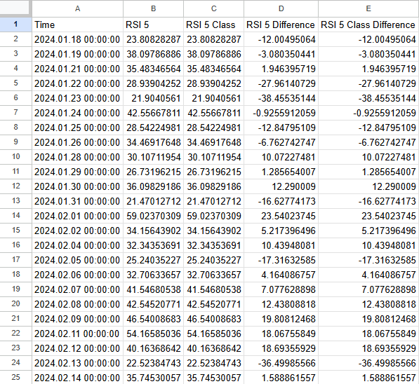
Fig 3: Our RSI class has passed our test, using it is identical to manually working with the RSI indicator class.

Now that we are confident in our implementation of the class, let us write out the class in a dedicated include file, so we can share the class with our Expert Advisor and any other exercises we conduct in future that may require the same set of functionality. When fully composed, this is what our class looks like in its current form.

//+------------------------------------------------------------------+
//|                                                          RSI.mqh |
//|                                               Gamuchirai Ndawana |
//|                    https://www.mql5.com/en/users/gamuchiraindawa |
//+------------------------------------------------------------------+
#property copyright "Gamuchirai Ndawana"
#property link      "https://www.mql5.com/en/users/gamuchiraindawa"
#property version   "1.00"

//+------------------------------------------------------------------+
//| This class will provide us with usefull functionality            |
//+------------------------------------------------------------------+
class RSI
  {
private:
   //--- Have the indicator values been copied to the buffer?
   bool              indicator_values_initialized;
   bool              indicator_differenced_values_initialized;

   //--- Give the user feedback
   string            user_feedback(int flag);

protected:
   //--- The handler for our RSI
   int               rsi_handler;
   //--- The Symbol our RSI should be applied on
   string            rsi_symbol;
   //--- Our RSI period
   int               rsi_period;
   //--- How far into the future we wish to forecast
   int               forecast_horizon;
   //--- The buffer for our RSI indicator
   double            rsi_reading[];
   vector            rsi_differenced_values;
   //--- The current size of the buffer the user last requested
   int               rsi_buffer_size;
   int               rsi_differenced_buffer_size;
   //--- The time frame our RSI should be applied on
   ENUM_TIMEFRAMES   rsi_time_frame;
   //--- The price should the RSI be applied on
   ENUM_APPLIED_PRICE rsi_price;

public:
                     RSI();
                     RSI(string user_symbol,ENUM_TIMEFRAMES user_time_frame,int user_period,ENUM_APPLIED_PRICE user_price);
                    ~RSI();
   bool              SetIndicatorValues(int buffer_size,bool set_as_series);
   bool              IsValid(void);
   double            GetCurrentReading(void);
   double            GetReadingAt(int index);
   bool              SetDifferencedIndicatorValues(int buffer_size,int differencing_period,bool set_as_series);
   double            GetDifferencedReadingAt(int index);
  };
//+------------------------------------------------------------------+
//| Our default constructor for our RSI class                        |
//+------------------------------------------------------------------+
void RSI::RSI()
  {
   indicator_values_initialized = false;
   rsi_symbol                   = "EURUSD";
   rsi_time_frame               = PERIOD_D1;
   rsi_period                   = 5;
   rsi_price                    = PRICE_CLOSE;
   rsi_handler                  = iRSI(rsi_symbol,rsi_time_frame,rsi_period,rsi_price);
//--- Give the user feedback on initilization
   Print(user_feedback(0));
//--- Remind the user they called the default constructor
   Print("Default Constructor Called: ",__FUNCSIG__," ",&this);
  }

//+------------------------------------------------------------------+
//| Our parametric constructor for our RSI class                     |
//+------------------------------------------------------------------+
void RSI::RSI(string user_symbol,ENUM_TIMEFRAMES user_time_frame,int user_period,ENUM_APPLIED_PRICE user_price)
  {
   indicator_values_initialized = false;
   rsi_symbol                   = user_symbol;
   rsi_time_frame               = user_time_frame;
   rsi_period                   = user_period;
   rsi_price                    = user_price;
   rsi_handler                  = iRSI(rsi_symbol,rsi_time_frame,rsi_period,rsi_price);
//--- Give the user feedback on initilization
   Print(user_feedback(0));
  }

//+------------------------------------------------------------------+
//| Our destructor for our RSI class                                 |
//+------------------------------------------------------------------+
void RSI::~RSI()
  {
//--- Free up resources we don't need and reset our flags
   if(IndicatorRelease(rsi_handler))
     {
      indicator_differenced_values_initialized = false;
      indicator_values_initialized = false;
      Print(user_feedback(5));
     }
  }

//+------------------------------------------------------------------+
//| Get our current reading from the RSI indicator                   |
//+------------------------------------------------------------------+
double RSI::GetCurrentReading(void)
  {
   double temp[];
   CopyBuffer(this.rsi_handler,0,0,1,temp);
   return(temp[0]);
  }

//+------------------------------------------------------------------+
//| Set our indicator values and our buffer size                     |
//+------------------------------------------------------------------+
bool              RSI::SetIndicatorValues(int buffer_size,bool set_as_series)
  {
   rsi_buffer_size = buffer_size;
   CopyBuffer(this.rsi_handler,0,0,buffer_size,rsi_reading);
   if(set_as_series)
      ArraySetAsSeries(this.rsi_reading,true);
   indicator_values_initialized = true;

//--- Did something go wrong?
   vector rsi_test;
   rsi_test.CopyIndicatorBuffer(rsi_handler,0,0,buffer_size);
   if(rsi_test.Sum() == 0)
      return(false);

//--- Everything went fine.
   return(true);
  }
//+--------------------------------------------------------------+
//| Let's set the conditions for our differenced data            |
//+--------------------------------------------------------------+
bool              RSI::SetDifferencedIndicatorValues(int buffer_size,int differencing_period,bool set_as_series)
  {
//--- Internal variables
   rsi_differenced_buffer_size = buffer_size;
   rsi_differenced_values = vector::Zeros(rsi_differenced_buffer_size);

//--- Prepare to record the differences in our RSI readings
   double temp_buffer[];
   int fetch = (rsi_differenced_buffer_size + (2 * differencing_period));
   CopyBuffer(rsi_handler,0,0,fetch,temp_buffer);
   if(set_as_series)
      ArraySetAsSeries(temp_buffer,true);

//--- Fill in our values iteratively
   for(int i = rsi_differenced_buffer_size;i > 1; i--)
     {
      rsi_differenced_values[i-1] = temp_buffer[i-1] - temp_buffer[i-1+differencing_period];
     }

//--- If the norm of a vector is 0, the vector is empty!
   if(rsi_differenced_values.Norm(VECTOR_NORM_P) != 0)
     {
      Print(user_feedback(2));
      indicator_differenced_values_initialized = true;
      return(true);
     }

   indicator_differenced_values_initialized = false;
   Print(user_feedback(3));
   return(false);
  }

 //--- Get a differenced value at a specific index
   double            RSI::GetDifferencedReadingAt(int index)
     {
      //--- Make sure we're not trying to call values beyond our index
      if(index > rsi_differenced_buffer_size)
        {
         Print(user_feedback(4));
         return(-1e10);
        }

      //--- Make sure our values have been set
      if(!indicator_differenced_values_initialized)
        {

         //--- The user is trying to use values before they were set in memory
         Print(user_feedback(1));
         return(-1e10);
        }

      //--- Return the differenced value of our indicator at a specific index
      if((indicator_differenced_values_initialized) && (index < rsi_differenced_buffer_size))
         return(rsi_differenced_values[index]);

      //--- Something went wrong.
      return(-1e10);
     }

//+------------------------------------------------------------------+
//| Get a reading at a specific index from our RSI buffer            |
//+------------------------------------------------------------------+
double            RSI::GetReadingAt(int index)
  {
//--- Is the user trying to call indexes beyond the buffer?
   if(index > rsi_buffer_size)
     {
      Print(user_feedback(4));
      return(-1e10);
     }

//--- Get the reading at the specified index
   if((indicator_values_initialized) && (index < rsi_buffer_size))
      return(rsi_reading[index]);

//--- User is trying to get values that were not set prior
   else
     {
      Print(user_feedback(1));
      return(-1e10);
     }
  }

//+------------------------------------------------------------------+
//| Check if our indicator handler is valid                          |
//+------------------------------------------------------------------+
bool RSI::IsValid(void)
  {
   return((this.rsi_handler != INVALID_HANDLE));
  }

//+------------------------------------------------------------------+
//| Give the user feedback on the actions he is performing           |
//+------------------------------------------------------------------+
string RSI::user_feedback(int flag)
  {
   string message;

//--- Check if the RSI indicator loaded correctly
   if(flag == 0)
     {
      //--- Check the indicator was loaded correctly
      if(IsValid())
         message = "RSI Indicator Class Loaded Correcrtly \nSymbol: " + (string) rsi_symbol + "\nPeriod: " + (string) rsi_period;
      return(message);
      //--- Something went wrong
      message = "Error loading RSI Indicator: [ERROR] " + (string) GetLastError();
      return(message);
     }

//--- User tried getting indicator values before setting them
   if(flag == 1)
     {
      message = "Please set the indicator values before trying to fetch them from memory, call SetIndicatorValues()";
      return(message);
     }

//--- We sueccessfully set our differenced indicator values
   if(flag == 2)
     {
      message = "Succesfully set differenced indicator values.";
      return(message);
     }

//--- Failed  to set our differenced indicator values
   if(flag == 3)
     {
      message = "Failed to set our differenced indicator values: [ERROR] " + (string) GetLastError();
      return(message);
     }

//--- The user is trying to retrieve an index beyond the buffer size and must update the buffer size first
   if(flag == 4)
     {
      message = "The user is attempting to use call an index beyond the buffer size, update the buffer size first";
      return(message);
     }

//--- The class has been deactivated by the user
   if(flag == 5)
     {
      message = "Goodbye.";
      return(message);
     }

//--- No feedback
   else
      return("");
  }
//+------------------------------------------------------------------+

Now let us fetch the market data we need using a collection of instances of our RSI class. We will store pointers to each instance of our class in an array of the custom type we have defined. MQL5 allows us to automatically generate objects on the fly as and when we need them. However, this flexibility comes at the price of having to always clean up after ourselves to prevent issues related to memory leakage.

//+------------------------------------------------------------------+
//|                                                      ProjectName |
//|                                      Copyright 2020, CompanyName |
//|                                       http://www.companyname.net |
//+------------------------------------------------------------------+
#property copyright "Copyright 2024, MetaQuotes Ltd."
#property link      "https://www.mql5.com"
#property version   "1.00"
#property script_show_inputs

//+------------------------------------------------------------------+
//| System constants                                                 |
//+------------------------------------------------------------------+
#define HORIZON 10

//+------------------------------------------------------------------+
//| Libraries                                                        |
//+------------------------------------------------------------------+
#include <VolatilityDoctor\Indicators\RSI.mqh>

//+------------------------------------------------------------------+
//| Global variables                                                 |
//+------------------------------------------------------------------+
RSI *my_rsi_array[14];
string file_name = Symbol() + " RSI Algorithmic Input Selection.csv";

//+------------------------------------------------------------------+
//| Inputs                                                           |
//+------------------------------------------------------------------+
input int size = 3000;

//+------------------------------------------------------------------+
//| Our script execution                                             |
//+------------------------------------------------------------------+
void OnStart()
  {
//--- How much data should we store in our indicator buffer?
   int fetch = size + (2 * HORIZON);

//--- Store pointers to our RSI objects
   for(int i = 0; i <= 13; i++)
     {
      //--- Create an RSI object
      my_rsi_array[i] = new RSI(Symbol(),PERIOD_CURRENT,((i+1) * 5),PRICE_CLOSE);
      //--- Set the RSI buffers
      my_rsi_array[i].SetIndicatorValues(fetch,true);
      my_rsi_array[i].SetDifferencedIndicatorValues(fetch,HORIZON,true);
     }

//---Write to file
   int file_handle=FileOpen(file_name,FILE_WRITE|FILE_ANSI|FILE_CSV,",");

   for(int i=size;i>=1;i--)
     {
      if(i == size)
        {
         FileWrite(file_handle,"Time","True Close","Open","High","Low","Close","RSI 5","RSI 10","RSI 15","RSI 20","RSI 25","RSI 30","RSI 35","RSI 40","RSI 45","RSI 50","RSI 55","RSI 60","RSI 65","RSI 70","Diff RSI 5","Diff RSI 10","Diff RSI 15","Diff RSI 20","Diff RSI 25","Diff RSI 30","Diff RSI 35","Diff RSI 40","Diff RSI 45","Diff RSI 50","Diff RSI 55","Diff RSI 60","Diff RSI 65","Diff RSI 70");
        }

      else
        {
         FileWrite(file_handle,
                   iTime(_Symbol,PERIOD_CURRENT,i),
                   iClose(_Symbol,PERIOD_CURRENT,i),
                   iOpen(_Symbol,PERIOD_CURRENT,i) - iOpen(Symbol(),PERIOD_CURRENT,i + HORIZON),
                   iHigh(_Symbol,PERIOD_CURRENT,i) - iHigh(Symbol(),PERIOD_CURRENT,i + HORIZON),
                   iLow(_Symbol,PERIOD_CURRENT,i) - iLow(Symbol(),PERIOD_CURRENT,i + HORIZON),
                   iClose(_Symbol,PERIOD_CURRENT,i) - iClose(Symbol(),PERIOD_CURRENT,i + HORIZON),
                   my_rsi_array[0].GetReadingAt(i),
                   my_rsi_array[1].GetReadingAt(i),
                   my_rsi_array[2].GetReadingAt(i),
                   my_rsi_array[3].GetReadingAt(i),
                   my_rsi_array[4].GetReadingAt(i),
                   my_rsi_array[5].GetReadingAt(i),
                   my_rsi_array[6].GetReadingAt(i),
                   my_rsi_array[7].GetReadingAt(i),
                   my_rsi_array[8].GetReadingAt(i),
                   my_rsi_array[9].GetReadingAt(i),
                   my_rsi_array[10].GetReadingAt(i),
                   my_rsi_array[11].GetReadingAt(i),
                   my_rsi_array[12].GetReadingAt(i),
                   my_rsi_array[13].GetReadingAt(i),
                   my_rsi_array[0].GetDifferencedReadingAt(i),
                   my_rsi_array[1].GetDifferencedReadingAt(i),
                   my_rsi_array[2].GetDifferencedReadingAt(i),
                   my_rsi_array[3].GetDifferencedReadingAt(i),
                   my_rsi_array[4].GetDifferencedReadingAt(i),
                   my_rsi_array[5].GetDifferencedReadingAt(i),
                   my_rsi_array[6].GetDifferencedReadingAt(i),
                   my_rsi_array[7].GetDifferencedReadingAt(i),
                   my_rsi_array[8].GetDifferencedReadingAt(i),
                   my_rsi_array[9].GetDifferencedReadingAt(i),
                   my_rsi_array[10].GetDifferencedReadingAt(i),
                   my_rsi_array[11].GetDifferencedReadingAt(i),
                   my_rsi_array[12].GetDifferencedReadingAt(i),
                   my_rsi_array[13].GetDifferencedReadingAt(i)
                  );
        }
     }
//--- Close the file
   FileClose(file_handle);

//--- Delete our RSI object pointers
   for(int i = 0; i <= 13; i++)
     {
      delete my_rsi_array[i];
     }
  }
//+------------------------------------------------------------------+
#undef HORIZON

Analyzing The Data In Python

We can now start analyzing the data we have collected from our MetaTrader 5 Terminal. Our first step will be to load the standard libraries we need.

import pandas as pd
import numpy as np
import seaborn as sns
import matplotlib.pyplot as plt
import plotly

Now read in the market data. Also, let us create a flag to denote if the current price level is greater than or less than the price that was offered 10 days ago. Recall that 10 days is the same period we used in our script to calculate the change in RSI levels.

#Let's read in our market data
data = pd.read_csv("EURUSD RSI Algorithmic Input Selection.csv")
data['Bull'] = np.NaN

data.loc[data['True Close'] > data['True Close'].shift(10),'Bull'] = 1
data.loc[data['True Close'] < data['True Close'].shift(10),'Bull'] = 0

data.dropna(inplace=True)
data.reset_index(inplace=True,drop=True)

We need to calculate the actual market returns as well.

#Estimate the market returns
#Define our forecast horizon
HORIZON = 10
data['Target'] = 0

data['Return'] = data['True Close'].shift(-HORIZON) - data['True Close']
data.loc[data['Return'] > 0,'Target'] = 1

#Drop missing values
data.dropna(inplace=True)

Most importantly, we need to delete all the data that overlaps with our intended back test period.

#No cheating boys.
_ = data.iloc[((-365 * 3) + 95):,:]
data = data.iloc[:((-365 * 3) + 95),:]
data

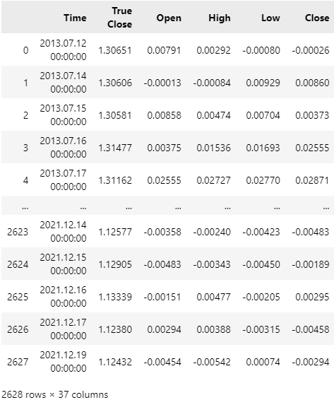
Fig 4: Our dataset no longer contains any of the dates that overlap with our back test period.

We can visualize the distribution of EURUSD 10 Day market returns, and we can quickly see that the market returns are fixed around 0. This general distribution shape comes as little surprise and is not unique to the EURUSD pair.

plt.title('Distribution of EURUSD 10 Day Returns')
plt.grid()
sns.histplot(data['Return'],color='black')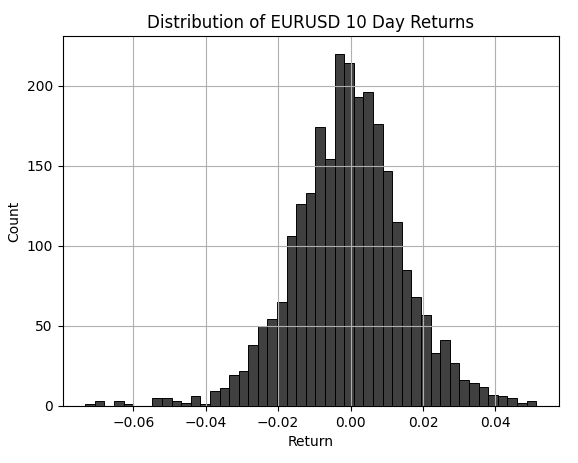

Fig 5: Visualizing the 10 Day EURUSD return distribution.

This exercise offers us a unique opportunity to visually see the difference between the distribution of RSI levels on a short period and RSI levels on a long period. The dashed vertical red lines, mark the standardized 30 and 70 levels. The black bars mark the distribution of the RSI levels when its period is set to 5. We can see the 5 period RSI will generate many signals past the standardized levels. However, the white bars, represent the distribution of RSI levels when the period is set to 70. We can visually see almost no signals will be generated at all. It is this change in the shape of the distribution that makes it challenging for algorithmic traders to always follow "best practices" for using an indicator.

plt.title('Comapring The Distribution of RSI Changes Across Different RSI Periods')
sns.histplot(data['RSI 5'],color='black')
sns.histplot(data['RSI 70'],color='white')
plt.xlabel('RSI Level')
plt.legend(['RSI 5','RSI 70'])
plt.axvline(30,color='red',linestyle='--')
plt.axvline(70,color='red',linestyle='--')
plt.grid()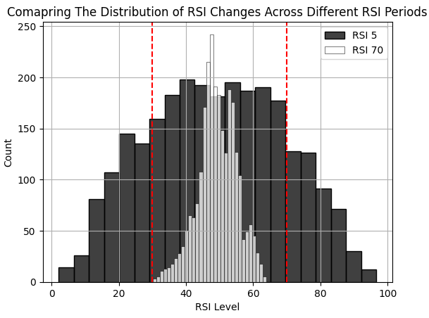

Fig 6: Comparing the distribution of RSI levels across different RSI periods.

Creating a scatter plot with the 10-period change in the 60 period RSI on both the x and y-axis, allows us to visualize whether there is a relationship between the change in the indicator and the target. It appears that a change of 10 RSI levels, may be a reasonable trading signal to go for short positions if the RSI reading fell by 10 levels. Or enter long positions if the RSI level increased by 10.

plt.title('Scatter Plot of 10 Day Change in 50 Period RSI & EURUSD 10 Day Return')
sns.scatterplot(data,y='Diff RSI 60',x='Diff RSI 60',hue='Target')
plt.xlabel('50 Period RSI')
plt.ylabel('50 Period RSI')
plt.grid()
plt.axvline(-10,color='red',linestyle='--')
plt.axvline(10,color='red',linestyle='--')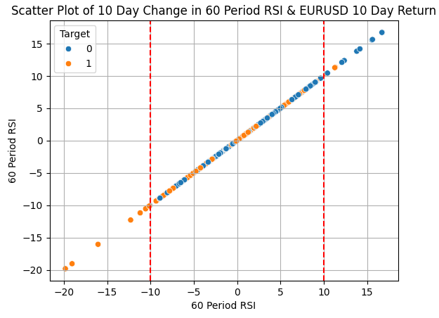

Fig 7: Visualizing the relationship between the change in the 60 Period RSI and the target.

Trying to combine the signals generated by changes on RSI with different periods may sound like a reasonable enough idea. However, it appears to do little in the way of better separating our two classes of interest.

plt.title('Scatter Plot of 10 Day Change in 5 Period RSI & EURUSD 10 Day Return')
sns.scatterplot(data,y='Diff RSI 60',x='Diff RSI 5',hue='Target')
plt.xlabel('5 Period RSI')
plt.ylabel('5 Period RSI')
plt.grid()

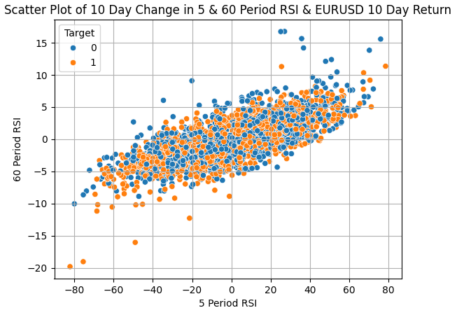
Fig 8: It appears that simply using RSI indicators with different periods is a poor source of confirmation.

We have 14 different RSI indicators to choose from. Instead of running 14 back tests to decide which period may serve us best, we can estimate the optimal period by evaluating the performance of a model trained with all 14 RSI indicators as its inputs and then evaluating the importance of features the statistical model learned from the data it was trained with.

Notice that, we always have the choice of employing statistical models for prediction accuracy, or for interpretations and insights. Today we are performing the latter. We will fit a Ridge model on the differences in all 14 RSI indicator inputs. The Ridge model has tuning parameters of its own. We will therefore perform a grid search over the input space for the Ridge statistical model. In particular, we will be adjusting the tuning parameters:

Alpha: The ridge model requires that a penalty added to control the model's coefficients.
Tolerance: Determines the smallest change necessary to set stopping conditions / other conditions for subroutines depending on the solver the user has selected.

For our discussion, we will be using a ridge model with the 'sparse_cg' solver. The reader is free to also consider tuning the model if they chose to.

The Ridge model is particularly helpful for us because it shrinks its coefficients down to 0 to reduce the model's loss. Therefore, we will search a wide space of initial settings for our model and then focus on the initial settings that brought about the lowest error. The configuration of the model's weights in its best performing mode can quickly inform us which RSI period our model depended on the most. In our particular example today, it was the 10-period change in the 55 period RSI that obtained the largest coefficients from our best performing model.

#Set the max levels we wish to check
ALPHA_LEVELS = 10
TOL_LEVELS   = 10

#DataFrame labels
r_c = 'TOL_LEVEL_'
r_r = 'ALHPA_LEVEL_'

results_columns = []
results_rows = []

for c in range(TOL_LEVELS):
    n_c = r_c + str(c)
    n_r = r_r + str(c)
    results_columns.append(n_c)
    results_rows.append(n_r)

#Create a DataFrame to store our results
results = pd.DataFrame(columns=results_columns,index=results_rows)

#Cross validate our model
for i in range(TOL_LEVELS):
    tol = 10 ** (-i)
    error = []
    for j in range(ALPHA_LEVELS):
        #Set alpha
        alpha = 10 ** (-j)
        
        #Its good practice to generally check the 0 case
        if(i == 0 & j == 0):
            model = Ridge(alpha=j,tol=i,solver='sparse_cg')

        #Otherwise use a float
        model = Ridge(alpha=alpha,tol=tol,solver='sparse_cg')

        #Store the error levels
        error.append(np.mean(np.abs(cross_val_score(model,data.loc[:,['Diff RSI 5',
       'Diff RSI 10', 'Diff RSI 15', 'Diff RSI 20', 'Diff RSI 25',
       'Diff RSI 30', 'Diff RSI 35', 'Diff RSI 40', 'Diff RSI 45',
       'Diff RSI 50', 'Diff RSI 55', 'Diff RSI 60', 'Diff RSI 65',
       'Diff RSI 70',]],data['Return'],cv=tscv))))
    
    #Record the error levels
    results.iloc[:,i] = error
    
results

The table below summarizes our results. We observe that, our lowest error rates were obtained when we set our model's initial parameters both set to 0.

Tuning Parameter	Model Error
ALHPA_LEVEL_0	0.053509
ALHPA_LEVEL_1	0.056245
ALHPA_LEVEL_2	0.060158
ALHPA_LEVEL_3	0.062230
ALHPA_LEVEL_4	0.061521
ALHPA_LEVEL_5	0.064312
ALHPA_LEVEL_6	0.073248
ALHPA_LEVEL_7	0.079310
ALHPA_LEVEL_8	0.081914
ALHPA_LEVEL_9	0.085171

It is also possible to visualize our findings using a contour plot. We want to use models in the region of the plot associated with low error, the blue regions. These are our best performing models so far. Let us now visualize the size of each coefficient in the model. The largest coefficient will be assigned to the input our model depended on the most.

import plotly.graph_objects as go

fig = go.Figure(data =
    go.Contour(
        z=results,
        colorscale='bluered'
    ))

fig.update_layout(
    width = 600,
    height = 400,
    title='Contour Plot Of Our Error Forecasting EURUSD Using Grid Search '
)

fig.show()

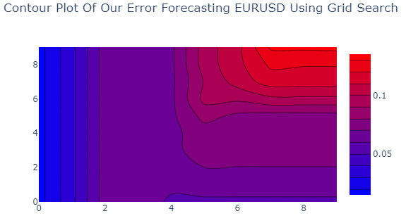
Fig 9: We have found optimal input settings for our Ridge model predicting the 10 day EURUSD return.

Plotting the data visually, we can quickly see the coefficient associated with the 55 Period RSI was assigned the largest absolute value. This gives us some confidence to narrow our focus down to that particular RSI setup.

#Let's visualize the importance of each column
model = Ridge(alpha=0,tol=0,solver='sparse_cg')

model.fit(data.loc[:,['Diff RSI 5',
       'Diff RSI 10', 'Diff RSI 15', 'Diff RSI 20', 'Diff RSI 25',
       'Diff RSI 30', 'Diff RSI 35', 'Diff RSI 40', 'Diff RSI 45',
       'Diff RSI 50', 'Diff RSI 55', 'Diff RSI 60', 'Diff RSI 65',
       'Diff RSI 70',]],data['Return'])

#Clearly our model relied on the 25 Period RSI the most, from all the data it had available at training
sns.barplot(np.abs(model.coef_),color='black')
plt.title('Rleative Feature Importance')
plt.ylabel('Coefficient Value')
plt.xlabel('Coefficient Index')
plt.grid()

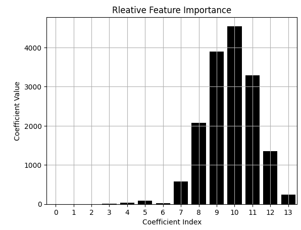
Fig 10: The coefficient associated with the Difference in the 55 Period RSI was assigned the largest value.

Now that we have identified our period of interest, let us also evaluate how the error of our model changes, as we cycle through increasing RSI levels of 10. We will create 3 additional columns in our data frame. Column 1 will have the value 1 if the RSI reading is greater than the first value we want to check. Otherwise, if the RSI reading is less than some particular value we wish to check, Column 2 will have the value 1. In any other case, column 3 will have the value 1.

def objective(x):
    data = pd.read_csv("EURUSD RSI Algorithmic Input Selection.csv")
    data['0'] = 0
    data['1'] = 0
    data['2'] = 0
    HORIZON = 10
    data['Return'] = data['True Close'].shift(-HORIZON) - data['True Close']
    data.dropna(subset=['Return'],inplace=True)
    data.iloc[data['Diff RSI 55'] > x[0],12] = 1
    data.iloc[data['Diff RSI 55'] < x[1],13] = 1
    data.iloc[(data['Diff RSI 55'] < x[0]) & (data['RSI 55'] > x[1]),14] = 1
    #Calculate or RMSE When using those levels
    model = Ridge(alpha=0,tol=0,solver='sparse_cg')
    error = np.mean(np.abs(cross_val_score(model,data.iloc[:,12:15],data['Return'],cv=tscv)))
    return(error)

Let us evaluate the error produced by our model if we set 0 to be our critical level.

#Bad rules for using the RSI
objective([0,0])

0.026897725573317266

If we input the 70 and 30 levels into our function, our error increases. We will perform a grid search in steps of 10, to find changes in RSI levels that are better suited for the 55 Period RSI. Our results found that the optimal change level appears close to 10 RSI levels.

#Bad rules for using the RSI
objective([70,30])

0.031258730612736006

LEVELS  = 10
results = []

for i in np.arange(0,(LEVELS)):
    results.append(objective([i * 10,-(i * 10)]))

plt.plot(results,color='black')
plt.ylabel('Error Rate')
plt.xlabel('Change in RSI as multiples of 10')
plt.grid()
plt.scatter(results.index(min(results)),min(results),color='red')
plt.title('Measuring The Strength of Changes In RSI Levels')

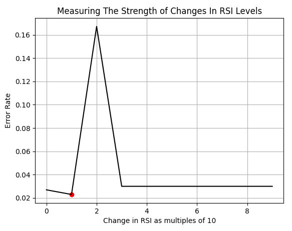
Fig 11: Visualizing the optimal change level in our RSI indicator.

Let us now perform another finer search, between the interval of RSI changes in the 0 and 20 range. Upon closer inspection, we observe that the true optima appears to be on the value 9. However, we do not conduct such exercises to fit historical data perfectly, that is called over fitting and is a bad practice. Our goal is not to perform an exercise in curve fitting. Instead of taking the optimal value exactly where it appears in our analysis of historical data, we embrace the fact that the location of the optima may change, and rather we aim to be within a certain fraction of a standard deviation away from the optimal value on either side to serve as our confidence intervals.

LEVELS  = 20
coef = 0.5
results = []

for i in np.arange(0,(LEVELS),1):
    results.append(objective([i,-(i)]))

plt.plot(results)
plt.ylabel('Error Rate')
plt.xlabel('Change in RSI')
plt.grid()
plt.scatter(results.index(min(results)),min(results),color='red')
plt.title('Measuring The Strength of Changes In RSI Levels')


plt.axvline(results.index(min(results)),color='red')
plt.axvline(results.index(min(results)) - (coef * np.std(data['Diff RSI 55'])),linestyle='--',color='red')
plt.axvline(results.index(min(results)) + (coef * np.std(data['Diff RSI 55'])),linestyle='--',color='red')

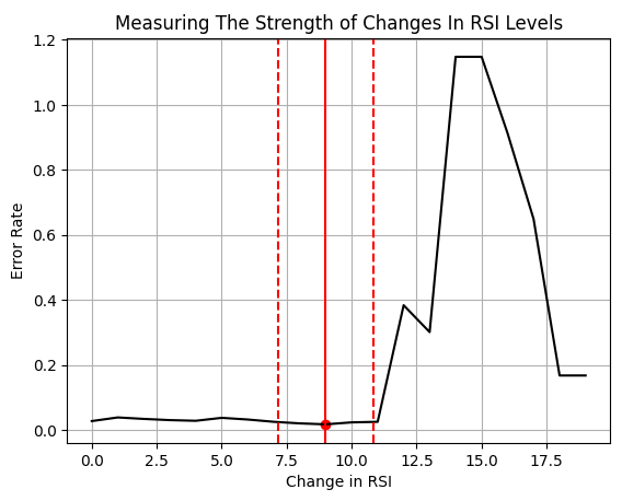
Fig 12: Visualizing the error rate associated with setting different thresholds for RSI level changes.

We can visually see the region we believe may be optimal overlaid on top of the historical distribution of change in the RSI changes.

sns.histplot(data['Diff RSI 55'],color='black')
coef = 0.5
plt.axvline((results.index(min(results))),linestyle='--',color='red')
plt.axvline(results.index(min(results)) - (coef * np.std(data['Diff RSI 55'])),color='red')
plt.axvline(results.index(min(results)) + (coef * np.std(data['Diff RSI 55'])),color='red')
plt.axvline(-(results.index(min(results))),linestyle='--',color='red')
plt.axvline(-(results.index(min(results)) - (coef * np.std(data['Diff RSI 55']))),color='red')
plt.axvline(-(results.index(min(results)) + (coef * np.std(data['Diff RSI 55']))),color='red')
plt.title("Visualizing our Optimal Point in The Distribution")

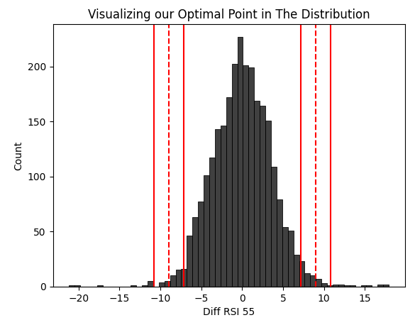
Fig 13: Visualizing the optimal regions we have selected for our RSI trading signals.

Let us get the values of our estimation of good confidence intervals, these will serve as the critical values in our Expert Advisor that trigger long and short signals.

results.index(min(results)) + ( coef * np.std(data['Diff RSI 55']))

10.822857254027287

And our lower bound.

results.index(min(results)) - (coef * np.std(data['Diff RSI 55']))

7.177142745972713

Let's obtain an explanation from our Ridge model to interpret the RSI indicator in a way we may not have intuitively thought of.

def explanation(x):
    data = pd.read_csv("EURUSD RSI Algorithmic Input Selection.csv")
    data['0'] = 0
    data['1'] = 0
    data['2'] = 0
    HORIZON = 10
    data['Return'] = data['True Close'].shift(-HORIZON) - data['True Close']
    data.dropna(subset=['Return'],inplace=True)
    data.iloc[data['Diff RSI 55'] > x[0],12] = 1
    data.iloc[data['Diff RSI 55'] < x[1],13] = 1
    data.iloc[(data['Diff RSI 55'] < x[0]) & (data['RSI 55'] > x[1]),14] = 1
    #Calculate or RMSE When using those levels
    model = Ridge(alpha=0,tol=0,solver='sparse_cg')
    model.fit(data.iloc[:,12:15],data['Return'])
    return(model.coef_.copy())

We see that, when the RSI indicator changes by more than 9, our optimal value, our model learned positive coefficients, which imply we should enter long positions. Otherwise, the model asserts we should sell under any other conditions.

opt = 9

print(explanation([opt,-opt]))

[ 1.97234840e-04 -1.64215118e-04 -7.55222156e-05]

Building Our Expert Advisor

Assuming our knowledge of the past, is a good model of the future, can we build an application to trade the EURUSD profitably using what we have now learned about the market? To get started, we will first define important system constants that we will need throughout our program and across any other versions we may build.

//+------------------------------------------------------------------+
//|                                  Algorithmic Input Selection.mq5 |
//|                                               Gamuchirai Ndawana |
//|                    https://www.mql5.com/en/users/gamuchiraindawa |
//+------------------------------------------------------------------+
#property copyright "Gamuchirai Ndawana"
#property link      "https://www.mql5.com/en/users/gamuchiraindawa"
#property version   "1.00"

//+------------------------------------------------------------------+
//| System constants                                                 |
//+------------------------------------------------------------------+
#define RSI_PERIOD 55
#define RSI_TIME_FRAME PERIOD_D1
#define SYSTEM_TIME_FRAME PERIOD_D1
#define RSI_PRICE  PRICE_CLOSE
#define RSI_BUFFER_SIZE 20
#define TRADING_VOLUME SymbolInfoDouble(Symbol(),SYMBOL_VOLUME_MIN)

Let's load our libraries.

//+------------------------------------------------------------------+
//| Load our RSI library                                             |
//+------------------------------------------------------------------+
#include <VolatilityDoctor\Indicators\RSI.mqh>
#include <Trade\Trade.mqh>

We will need a few global variables.

//+------------------------------------------------------------------+
//| Global variables                                                 |
//+------------------------------------------------------------------+
CTrade Trade;
RSI    rsi_55(Symbol(),RSI_TIME_FRAME,RSI_PERIOD,RSI_PRICE);
double last_value;
int    count;
int    ma_o_handler,ma_c_handler;
double ma_o[],ma_c[];
double trade_sl;

Our event handlers will each call their own dedicated method to handle the sub processes needed to complete their tasks.

//+------------------------------------------------------------------+
//| Expert initialization function                                   |
//+------------------------------------------------------------------+
int OnInit()
  {
//---
   setup();
//---
   return(INIT_SUCCEEDED);
  }
//+------------------------------------------------------------------+
//| Expert deinitialization function                                 |
//+------------------------------------------------------------------+
void OnDeinit(const int reason)
  {
//---
   IndicatorRelease(ma_c_handler);
   IndicatorRelease(ma_o_handler);
  }
//+------------------------------------------------------------------+
//| Expert tick function                                             |
//+------------------------------------------------------------------+
void OnTick()
  {
//---
   update();
  }
//+------------------------------------------------------------------+

The update function updates all our system variables and checks if we have to either open a position, or manage our open positions.

//+------------------------------------------------------------------+
//| Update our system variables                                      |
//+------------------------------------------------------------------+
void update(void)
  {
   static datetime time_stamp;
   datetime current_time = iTime(Symbol(),SYSTEM_TIME_FRAME,0);

   if(time_stamp != current_time)
     {
      time_stamp = current_time;
      CopyBuffer(ma_c_handler,0,0,1,ma_c);
      CopyBuffer(ma_o_handler,0,0,1,ma_o);

      if((count == 0) && (PositionsTotal() == 0))
        {
         rsi_55.SetIndicatorValues(RSI_BUFFER_SIZE,true);
         last_value = rsi_55.GetReadingAt(RSI_BUFFER_SIZE - 1);
         count = 1;
        }

      if(PositionsTotal() == 0)
         check_signal();

      if(PositionsTotal() > 0)
         manage_setup();
     }
  }

Our positions need to have their stop losses constantly adjusted to ensure that we reduce our risk levels whenever possible.

//+------------------------------------------------------------------+
//| Manage our open trades                                           |
//+------------------------------------------------------------------+
void manage_setup(void)
  {
   double bid = SymbolInfoDouble(Symbol(),SYMBOL_BID);
   double ask = SymbolInfoDouble(Symbol(),SYMBOL_ASK);

   if(PositionSelect(Symbol()))
     {
      double current_sl = PositionGetDouble(POSITION_SL);
      double current_tp = PositionGetDouble(POSITION_TP);
      double new_sl = (current_tp > current_sl) ? (bid-trade_sl) : (ask+trade_sl);
      double new_tp = (current_tp < current_sl) ? (bid+trade_sl) : (ask-trade_sl);
      //--- Buy setup
      if((current_tp > current_sl) && (new_sl < current_sl))
         Trade.PositionModify(Symbol(),new_sl,new_tp);

      //--- Sell setup
      if((current_tp < current_sl) && (new_sl > current_sl))
         Trade.PositionModify(Symbol(),new_sl,new_tp);
     }
  }

Our setup function is responsible for getting our system started up from the ground. It will prepare the indicators we need, and resets our counters.

//+------------------------------------------------------------------+
//| Setup our global variables                                       |
//+------------------------------------------------------------------+
void setup(void)
  {
   ma_c_handler = iMA(Symbol(),SYSTEM_TIME_FRAME,2,0,MODE_EMA,PRICE_CLOSE);
   ma_o_handler = iMA(Symbol(),SYSTEM_TIME_FRAME,2,0,MODE_EMA,PRICE_OPEN);
   count        = 0;
   last_value   = 0;
   trade_sl     = 1.5e-2;
  }

Lastly, our trading rules have been generated thanks to the coefficient values our model learned from the training data. This is the last function we will define before we undefine the system variables we created at the beginning of our program.

//+------------------------------------------------------------------+
//| Check if we have a trading setup                                 |
//+------------------------------------------------------------------+
void check_signal(void)
  {
   double current_reading = rsi_55.GetCurrentReading();
   Comment("Last Reading: ",last_value,"\nDifference in Reading: ",(last_value - current_reading));
   double bid = SymbolInfoDouble(Symbol(),SYMBOL_BID);
   double ask = SymbolInfoDouble(Symbol(),SYMBOL_ASK);
   double cp_lb = 7.17;
   double cp_ub = 10.82;

   if((((last_value - current_reading) <= -(cp_lb)) && ((last_value - current_reading) > (cp_ub)))|| ((((last_value - current_reading) > -(cp_lb))) && ((last_value - current_reading) < (cp_lb))))
     {
      if(ma_o[0] > ma_c[0])
        {
         if(PositionsTotal() == 0)
           {
            Trade.Sell(TRADING_VOLUME,Symbol(),bid,(ask+trade_sl),(ask-trade_sl));
            count = 0;
           }
        }
     }

   if(((last_value - current_reading) >= (cp_lb)) < ((last_value - current_reading) < cp_ub))
     {
      if(ma_c[0] < ma_o[0])
        {
         if(PositionsTotal() == 0)
           {
            Trade.Buy(TRADING_VOLUME,Symbol(),ask,(bid-trade_sl),(bid+trade_sl));
            count = 0;
           }
        }
     }
  }
//+------------------------------------------------------------------+

#undef RSI_BUFFER_SIZE
#undef RSI_PERIOD
#undef RSI_PRICE
#undef RSI_TIME_FRAME
#undef SYSTEM_TIME_FRAME
#undef TRADING_VOLUME
//+------------------------------------------------------------------+

Let us now get started with our back test of the trading system. Recall that in Fig 4, we deleted all the data that overlaps with our back test. Therefore, this may serve us as a close approximation of how our strategy may perform in real time. We will perform a 3-year back test of our strategy on Daily data, from 1 January 2022 until March 2025.

Our dates

Fig 14: The dates we will use for our back test of the trading strategy.

For best results, we always use "Every tick based on real ticks" because it renders the most accurate simulation of past market conditions based on the historical ticks the MetaTrader 5 Terminal collected on your behalf from your broker.

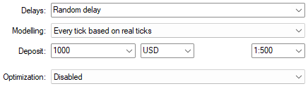
Fig 15: The conditions which we will perform our tests under matter a lot, and change the profitability of our strategy.

The equity curve produced by our strategy tester appears promising. But, let's interpret the detailed statistics together, to obtain a complete view of our strategy's performance.

Fig 16: The equity curve produced by EURUSD 55 Period RSI trading strategy.

Running our strategy produced the following statistics in our strategy tester:

Sharpe Ratio: 0.92
Expected payoff: 2.49
Total Net Profit: $151.87
Profit trades: 57.38%

However, pay attention to the fact that from the 61 total trades placed, only 4 were long trades. Why is our strategy so disproportionally biased towards selling? How can we correct this bias? Let us take another look at our EURUSD chart and try to make sense of this together.

Our back test

Fig 17: The detailed statistics of our Expert Advisor's historical performance on the Daily EURUSD Exchange Rate.

Improving Our Expert Advisor

In Fig 18, I have attached a screenshot of the Monthly EURUSD exchange rate. The 2 red vertical lines mark the beginning of the year 2009 and the end of the year 2021 respectively. The green vertical line, represents the beginning of the training data we used for our statistical model. One can quickly see why the model learned a bias for short positions, given the sustained bear trend that started in 2008.

Fig 18: Understanding why our model learned such bearish sentiment.

We do not always need more historical data, to try and correct for this. Rather, we can fit a more flexible model than the Ridge model we started with. The stronger learner, will then supply our strategy with additional long signals.

It is possible for us to give our Expert Advisor a reasonable idea of the probability that the exchange rate will rise over the next 10 Days. We can train a Random Forest Regressor to predict the probability that we will observe bullish price action. When the expected probability exceeds 0.5, our Expert Advisor will enter a long position. Otherwise, we will follow the strategy we learned from our Ridge model.

Modelling Probabilities in Python

To get started with our corrections, we will first import a few libraries.

from sklearn.metrics import accuracy_score
from sklearn.ensemble import RandomForestRegressor

Then we shall define our dependent and independent variables.

#Independent variable
X = data[['Diff RSI 55']]
#Dependent variable
y = data['Target']

Fit the model.

model = RandomForestRegressor()
model.fit(X,y)

Get ready to export to ONNX.

import onnx
from skl2onnx import convert_sklearn
from skl2onnx.common.data_types import FloatTensorType

Define the input shapes.

inital_params = [("float_input",FloatTensorType([1,1]))]

Create ONNX prototype and save it to disk.

onnx_proto = convert_sklearn(model=model,initial_types=inital_params,target_opset=12)
onnx.save(onnx_proto,"EURUSD Diff RSI 55 D1 1 1.onnx")

You can also visualize your model using the netron library, to ensure the right input and output attributes were given to your ONNX model.

import netron
netron.start("EURUSD Diff RSI 55 D1 1 1.onnx")

This is a graphical representation of our Random Forest Regressor and the attributes the model has. Netron can also be used to visualize Neural Networks and many other types of ONNX models.

ONNX Model

Fig 19: Visualizing our ONNX Random Forest Regressor model.

The inputs and output shapes were correctly specified by ONNX, so we can now move on to applying the Random Forest Regressor to help our Expert Advisor predict the probability of Bullish Price action happening over the next 10 days.

ONNX Model Details

Fig 20: The details of our ONNX model match the expected specifications we wanted to check for.

Improving Our Expert Advisor

Now that we have exported a probabilistic model of the EURUSD market, we can import our ONNX model into our Expert Advisor.

//+------------------------------------------------------------------+
//|                                  Algorithmic Input Selection.mq5 |
//|                                               Gamuchirai Ndawana |
//|                    https://www.mql5.com/en/users/gamuchiraindawa |
//+------------------------------------------------------------------+
#property copyright "Gamuchirai Ndawana"
#property link      "https://www.mql5.com/en/users/gamuchiraindawa"
#property version   "1.00"

//+------------------------------------------------------------------+
//| System resources                                                 |
//+------------------------------------------------------------------+
#resource "\\Files\\EURUSD Diff RSI 55 D1 1 1.onnx" as uchar onnx_model_buffer[];

We will also need a few new macros specifying the shape of our ONNX model.

#define ONNX_INPUTS 1
#define ONNX_OUTPUTS 1

Additionally, the ONNX model deserves a few global variables because we may quickly need them in several parts of our code.

long   onnx_model;
vectorf onnx_output(1);
vectorf onnx_input(1);

In the code snippet below, we have excluded parts of the code base that hasn't changed, and only show the changes made to initialize the ONNX model and set its parameter shapes.

//+------------------------------------------------------------------+
//| Setup our global variables                                       |
//+------------------------------------------------------------------+
bool setup(void)
  {
//--- Setup our technical indicators
  ...

//--- Create our ONNX model
   onnx_model = OnnxCreateFromBuffer(onnx_model_buffer,ONNX_DATA_TYPE_FLOAT);

//--- Validate the ONNX model
   if(onnx_model == INVALID_HANDLE)
     {
      return(false);
     }

//--- Define the I/O signature
   ulong onnx_param[] =  {1,1};

   if(!OnnxSetInputShape(onnx_model,0,onnx_param))
      return(false);

   if(!OnnxSetOutputShape(onnx_model,0,onnx_param))
      return(false);

   return(true);
  }

Additionally, our check for valid trading has been trimmed to only highlight the additional code added to it, and avoid duplicating the same code.

//+------------------------------------------------------------------+
//| Check if we have a trading setup                                 |
//+------------------------------------------------------------------+
void check_signal(void)
  {
   rsi_55.SetDifferencedIndicatorValues(RSI_BUFFER_SIZE,HORIZON,true);
   onnx_input[0] = (float) rsi_55.GetDifferencedReadingAt(RSI_BUFFER_SIZE - 1);

//--- Our Random forest model
   if(!OnnxRun(onnx_model,ONNX_DATA_TYPE_FLOAT,onnx_input,onnx_output))
      Comment("Failed to obtain a forecast from our model!");

   else
     {
      if(onnx_output[0] > 0.5)
         if(ma_o[0] < ma_c[0])
            Trade.Buy(TRADING_VOLUME,Symbol(),ask,(bid-trade_sl),(bid+trade_sl));
      Print("Model Bullish Probabilty: ",onnx_output);
     }
}

All in all, this is what our second version of the trading strategy looks like when fully composed.

//+------------------------------------------------------------------+
//|                                  Algorithmic Input Selection.mq5 |
//|                                               Gamuchirai Ndawana |
//|                    https://www.mql5.com/en/users/gamuchiraindawa |
//+------------------------------------------------------------------+
#property copyright "Gamuchirai Ndawana"
#property link      "https://www.mql5.com/en/users/gamuchiraindawa"
#property version   "1.00"

//+------------------------------------------------------------------+
//| System resources                                                 |
//+------------------------------------------------------------------+
#resource "\\Files\\EURUSD Diff RSI 55 D1 1 1.onnx" as uchar onnx_model_buffer[];

//+------------------------------------------------------------------+
//| System constants                                                 |
//+------------------------------------------------------------------+
#define RSI_PERIOD 55
#define RSI_TIME_FRAME PERIOD_D1
#define SYSTEM_TIME_FRAME PERIOD_D1
#define RSI_PRICE  PRICE_CLOSE
#define RSI_BUFFER_SIZE 20
#define TRADING_VOLUME SymbolInfoDouble(Symbol(),SYMBOL_VOLUME_MIN)
#define ONNX_INPUTS 1
#define ONNX_OUTPUTS 1
#define HORIZON 10

//+------------------------------------------------------------------+
//| Load our RSI library                                             |
//+------------------------------------------------------------------+
#include <VolatilityDoctor\Indicators\RSI.mqh>
#include <Trade\Trade.mqh>

//+------------------------------------------------------------------+
//| Global variables                                                 |
//+------------------------------------------------------------------+
CTrade Trade;
RSI    rsi_55(Symbol(),RSI_TIME_FRAME,RSI_PERIOD,RSI_PRICE);
double last_value;
int    count;
int    ma_o_handler,ma_c_handler;
double ma_o[],ma_c[];
double trade_sl;
long   onnx_model;
vectorf onnx_output(1);
vectorf onnx_input(1);

//+------------------------------------------------------------------+
//| Expert initialization function                                   |
//+------------------------------------------------------------------+
int OnInit()
  {
//---
   setup();
//---
   return(INIT_SUCCEEDED);
  }
//+------------------------------------------------------------------+
//| Expert deinitialization function                                 |
//+------------------------------------------------------------------+
void OnDeinit(const int reason)
  {
//---
   IndicatorRelease(ma_c_handler);
   IndicatorRelease(ma_o_handler);
  }
//+------------------------------------------------------------------+
//| Expert tick function                                             |
//+------------------------------------------------------------------+
void OnTick()
  {
//---
   update();
  }
//+------------------------------------------------------------------+

//+------------------------------------------------------------------+
//| Update our system variables                                      |
//+------------------------------------------------------------------+
void update(void)
  {
   static datetime time_stamp;
   datetime current_time = iTime(Symbol(),SYSTEM_TIME_FRAME,0);

   if(time_stamp != current_time)
     {
      time_stamp = current_time;
      CopyBuffer(ma_c_handler,0,0,1,ma_c);
      CopyBuffer(ma_o_handler,0,0,1,ma_o);

      if((count == 0) && (PositionsTotal() == 0))
        {
         rsi_55.SetIndicatorValues(RSI_BUFFER_SIZE,true);
         rsi_55.SetDifferencedIndicatorValues(RSI_BUFFER_SIZE,HORIZON,true);
         last_value = rsi_55.GetReadingAt(RSI_BUFFER_SIZE - 1);
         count = 1;
        }

      if(PositionsTotal() == 0)
         check_signal();

      if(PositionsTotal() > 0)
         manage_setup();
     }
  }

//+------------------------------------------------------------------+
//| Manage our open trades                                           |
//+------------------------------------------------------------------+
void manage_setup(void)
  {
   double bid = SymbolInfoDouble(Symbol(),SYMBOL_BID);
   double ask = SymbolInfoDouble(Symbol(),SYMBOL_ASK);

   if(PositionSelect(Symbol()))
     {
      double current_sl = PositionGetDouble(POSITION_SL);
      double current_tp = PositionGetDouble(POSITION_TP);
      double new_sl = (current_tp > current_sl) ? (bid-trade_sl) : (ask+trade_sl);
      double new_tp = (current_tp < current_sl) ? (bid+trade_sl) : (ask-trade_sl);
      //--- Buy setup
      if((current_tp > current_sl) && (new_sl < current_sl))
         Trade.PositionModify(Symbol(),new_sl,new_tp);

      //--- Sell setup
      if((current_tp < current_sl) && (new_sl > current_sl))
         Trade.PositionModify(Symbol(),new_sl,new_tp);
     }
  }

//+------------------------------------------------------------------+
//| Setup our global variables                                       |
//+------------------------------------------------------------------+
bool setup(void)
  {
//--- Setup our technical indicators
   ma_c_handler = iMA(Symbol(),SYSTEM_TIME_FRAME,2,0,MODE_EMA,PRICE_CLOSE);
   ma_o_handler = iMA(Symbol(),SYSTEM_TIME_FRAME,2,0,MODE_EMA,PRICE_OPEN);
   count        = 0;
   last_value   = 0;
   trade_sl     = 1.5e-2;

//--- Create our ONNX model
   onnx_model = OnnxCreateFromBuffer(onnx_model_buffer,ONNX_DATA_TYPE_FLOAT);

//--- Validate the ONNX model
   if(onnx_model == INVALID_HANDLE)
     {
      return(false);
     }

//--- Define the I/O signature
   ulong onnx_param[] =  {1,1};

   if(!OnnxSetInputShape(onnx_model,0,onnx_param))
      return(false);

   if(!OnnxSetOutputShape(onnx_model,0,onnx_param))
      return(false);

   return(true);
  }

//+------------------------------------------------------------------+
//| Check if we have a trading setup                                 |
//+------------------------------------------------------------------+
void check_signal(void)
  {
   rsi_55.SetDifferencedIndicatorValues(RSI_BUFFER_SIZE,HORIZON,true);
   last_value = rsi_55.GetReadingAt(RSI_BUFFER_SIZE - 1);

   double current_reading = rsi_55.GetCurrentReading();
   Comment("Last Reading: ",last_value,"\nDifference in Reading: ",(last_value - current_reading));
   double bid = SymbolInfoDouble(Symbol(),SYMBOL_BID);
   double ask = SymbolInfoDouble(Symbol(),SYMBOL_ASK);
   double cp_lb = 7.17;
   double cp_ub = 10.82;
   onnx_input[0] = (float) rsi_55.GetDifferencedReadingAt(RSI_BUFFER_SIZE - 1);

//--- Our Random forest model
   if(!OnnxRun(onnx_model,ONNX_DATA_TYPE_FLOAT,onnx_input,onnx_output))
      Comment("Failed to obtain a forecast from our model!");

   else
     {
      if(onnx_output[0] > 0.5)
         if(ma_o[0] < ma_c[0])
            Trade.Buy(TRADING_VOLUME,Symbol(),ask,(bid-trade_sl),(bid+trade_sl));
      Print("Model Bullish Probabilty: ",onnx_output);
     }

//--- The trading rules we learned from our Ridge Regression Model
//--- Ridge Regression Sell
   if((((last_value - current_reading) <= -(cp_lb)) && ((last_value - current_reading) > (cp_ub)))|| ((((last_value - current_reading) > -(cp_lb))) && ((last_value - current_reading) < (cp_lb))))
     {
      if(ma_o[0] > ma_c[0])
        {
         if(PositionsTotal() == 0)
           {
            Trade.Sell(TRADING_VOLUME,Symbol(),bid,(ask+trade_sl),(ask-trade_sl));
            count = 0;
           }
        }
     }
//--- Ridge Regression Buy
   else
      if(((last_value - current_reading) >= (cp_lb)) < ((last_value - current_reading) < cp_ub))
        {
         if(ma_c[0] < ma_o[0])
           {
            if(PositionsTotal() == 0)
              {
               Trade.Buy(TRADING_VOLUME,Symbol(),ask,(bid-trade_sl),(bid+trade_sl));
               count = 0;
              }
           }
        }
  }
//+------------------------------------------------------------------+

#undef RSI_BUFFER_SIZE
#undef RSI_PERIOD
#undef RSI_PRICE
#undef RSI_TIME_FRAME
#undef SYSTEM_TIME_FRAME
#undef TRADING_VOLUME
#undef ONNX_INPUTS
#undef ONNX_OUTPUTS
//+------------------------------------------------------------------+

We will be testing the strategy under the same conditions highlighted in Fig 14 and Fig 15. Here are the results we obtained with the second version of our trading strategy. The equity curve produced by our second version of the trading appears to be quite the same as the first equity curve we produced.

Fig 21: Visualizing the profitability of our second trading strategy.

It is only when we view the detailed statistics, that the differences between the two strategies start to surface. Our Sharpe ratio and expected payoff fell. Our new strategy placed 85 trades that's 39% more than the 61 trades placed by our initial strategy. Additionally, our total number of long positions increased from just 4 in the initial test, to 42 in our second test. That is an increase of 950%. So when we consider the amount of additional risk we are taking on is significant and yet, our accuracy and profitability statistics are only dropping marginally, then we start to build positive expectations about using the strategy. In our previous test, 57.38 of all our trades were profitable, and now 56.47%, that's a reduction of in accuracy of approximately 1.59%.

Fig 22: Our detailed statistics of the performance of our revised version of our trading strategy.

Conclusion

After reading this article, the reader walks away with an understanding of how they could employ grid search techniques alongside statistical models to help them select an optimal period to use for indicators without having to perform multiple back tests and manually search every single possible period. Additionally, the reader has also learned one possible way of estimating and comparing the value of new RSI levels they wish to trade, against the value of the traditional 70 and 30 levels, allowing the reader to trade adversarial market conditions with renewed confidence in their ability.

File Name	Description
Algorithmic Inputs Selection.ipynb	The Jupyter Notebook we used to perform numerical analysis using Python.
EURUSD Testing RSI Class.mql5	The MQL5 script we used to test our implementation of our custom RSI Class.
EURUSD RSI Algorithmic Input Selection.mql5	The script we used to fetch historical market data.
Algorithmic Input Selection.mql5	Our initial version of the Trading Strategy we built.
Algorithmic Input Selection 2.mql5	Our refined version of the Trading Strategy that corrected the bias learned by our initial trading strategy.