
Build Self Optimizing Expert Advisors in MQL5 (Part 6): Stop Out Prevention

It is possible for traders to correctly predict the future change in price of a market, but close their positions in a loss. In trading circles, this is commonly referred to as “Getting stopped out”. This problem arises from the fact that price levels do not change in straight and predictable lines.
In Fig 1, we have provided you with a snapshot of the hourly change in price of the EURUSD pair. The white, dashed vertical lines, mark the beginning and end of the trading day. A trader, who was confident that price levels were going to fall that day, would’ve correctly predicted the future change in price. Unfortunately, price levels rose considerably, before they fell, meaning that if our trader’s stop loss was within the red zone highlighted in Fig 1, he would’ve closed his position in loss, after correctly predicting the future change in price.

Fig 1: Visualizing situations in which traders typically get stopped out
Over the years, traders have suggested various solutions on how to solve this problem, but as we shall see through our discussion, most of these aren’t valid solutions. The most commonly cited solution is to simply “widen your stops”.
This implies that, traders should make their stop losses wider on particularly volatile trading days, to prevent getting stopped out. But this is bad advice because it encourages traders to form a habit of taking varying amounts of risk on similar trades, without any set and well-defined rules guiding their decision-making.
Another commonly cited solution is to “wait for confirmation before entering your trades”. Again, this is poor advice given the nature of the problem we are focused on. One may find out that waiting for confirmation only postpones the process of getting stopped out, and doesn’t solve the problem entirely.
In short, the problem of getting stopped out makes it challenging for traders to follow sound risk management principles, while at the same time reducing the profitability of trading sessions among other points of concern it creates for traders.
Therefore, we shall make it our goal, to equip you, the reader, with more reasonable and well-defined rules to minimize the frequency with which you get stopped out of your winning trades.
Our proposed solution will go against the grain of commonly cited solutions and will encourage you to build sound trading habits, such as keeping the size of your stop loss fixed, as opposed to the commonly cited solution of “widen your stop loss”.
Overview Of The Trading Strategy
Our trading strategy will be a mean reverting strategy, composed of a combination of support and resistance levels alongside technical analysis. We will first mark our price levels of interest using the previous day high and low. From there, we will wait to see if the previous day price levels will be broken during the present day. If for example the previous day high price is broken by a new high price during the current day, we will look for opportunities to occupy short positions in the market, betting that price levels will return to their average. The signal to enter short positions will clear for us when we observe price levels closing above the moving average indicator, after successfully closing above the previous high.
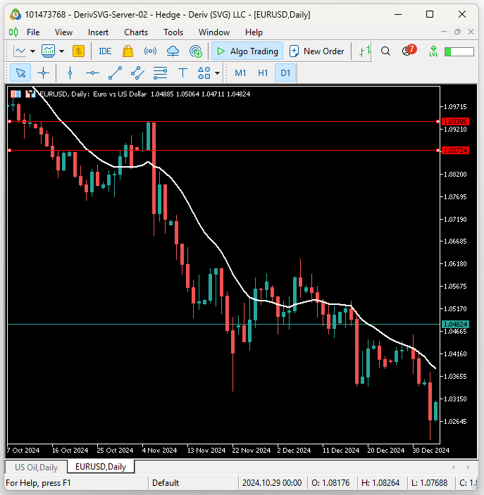
Fig 2: Visualizing our trading strategy in action
Overview of The Back test Period
To analyze the effectiveness of our proposed changes to the trading strategy, we must first have a fixed period over which we will compare the changes we are making to our system. For this discussion, we will begin our test from the first of January 2022 until the 1st of January 2025. The period in question has been highlighted in Fig 1, note that in the figure we are observing the EURUSD on the monthly time frame.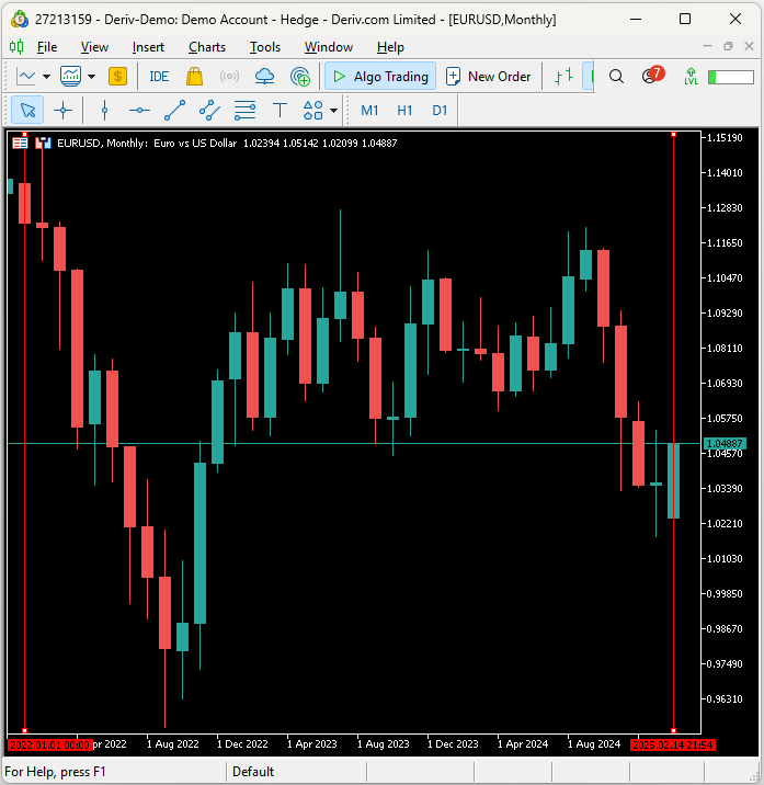
Fig 3: The period over which we will perform our back test
Our actual tests will be performed on the M30 time frame. In Fig 2 we have highlighted the intended market we will use for our tests, as well as the time period we discussed previously. These settings will be fixed throughout the remainder of the article, and hence the need for us to discuss them here. For all of our tests that are to follow, we will leave these settings unchanged. Additionally, be sure to select the EURUSD if you want to follow along with us, or whichever Symbol you prefer trading.
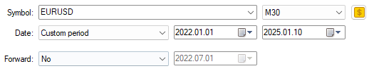
Fig 4: Our back test period
Additionally, select "Every tick based on real ticks" to reproduce the most accurate emulation of historic market events that we can create. Note that, this setting will fetch the relevant data from your broker, and this may take a considerable amount of time depending on your network provision.
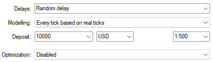
Fig 5: The account settings we will use for our back test
Getting Started in MQL5
Now that we have familiarized ourselves with the back test period for our test today, let us first establish a baseline measurement that we will surpass. We will begin by building a trading application to implement a support and resistance trading strategy that aims to trade breakouts. First, we shall import the trade library.
//+------------------------------------------------------------------+
//|                                               Baseline Model.mq5 |
//|                                               Gamuchirai Ndawana |
//|                    https://www.mql5.com/en/users/gamuchiraindawa |
//+------------------------------------------------------------------+
#property copyright "Gamuchirai Ndawana"
#property link      "https://www.mql5.com/en/users/gamuchiraindawa"
#property version   "1.00"

//+------------------------------------------------------------------+
//| Libraries                                                        |
//+------------------------------------------------------------------+
#include <Trade/Trade.mqh>
CTrade Trade;
Define system constants. These constants help us ensure that we have definite control over the behavior of our application across all tests.
//+------------------------------------------------------------------+
//| System constants                                                 |
//+------------------------------------------------------------------+
#define MA_PERIOD 14                //--- Moving Average Period
#define MA_TYPE   MODE_EMA          //--- Type of moving average we have
#define MA_PRICE PRICE_CLOSE        //---- Applied Price of Moving Average
#define TF_1 PERIOD_D1              //--- Our time frame for technical analysis
#define TF_2 PERIOD_M30             //--- Our time frame for managing positions
#define VOL 0.1                     //--- Our trading volume
#define SL_SIZE  1e3 * _Point       //--- The size of our stop loss
We will also need a few global variables to help us keep track of yesterday's price levels of interest.
//+------------------------------------------------------------------+
//| Our global variables                                             |
//+------------------------------------------------------------------+
int ma_handler,system_state;
double ma[];
double bid,ask,yesterday_high,yesterday_low;
const string last_high = "LAST_HIGH";
const string last_low = "LAST_LOW";
When our application has been loaded for the first time, setup all our technical indicators.
//+------------------------------------------------------------------+
//| Expert initialization function                                   |
//+------------------------------------------------------------------+
int OnInit()
  {
//---
   setup();
//---
   return(INIT_SUCCEEDED);
  }
If our application is no longer in us, release the technical indicators we are no longer using.
//+------------------------------------------------------------------+
//| Expert deinitialization function                                 |
//+------------------------------------------------------------------+
void OnDeinit(const int reason)
  {
//---
   release();
  }
If we ever receive updated prices, store them and also recalculate our indicator values.
//+------------------------------------------------------------------+
//| Expert tick function                                             |
//+------------------------------------------------------------------+
void OnTick()
  {
//---
   update();
  }
We shall now define each of the functions we have called in our event cycle. First, our update function will work on 2 different time frames. We have routines and procedures that must be performed once a day, and others must be performed over much shorter intervals. This separation of concerns is taken care of for us by the 2 system constants we defined, TF_1 (Daily Time Frame) and TF_2 (M30 Time Frame). Tasks such as fetching the previous day, high and low, need only to be done once a day. On the other hand, tasks, such as searching for positions, need only to be done once every new 30 min candle.
//+------------------------------------------------------------------+
//| Perform our update routines                                      |
//+------------------------------------------------------------------+
void update()
  {
//--- Daily procedures
     {
      static datetime time_stamp;
      datetime current_time = iTime(Symbol(),TF_1,0);
      if(time_stamp != current_time)
        {
         yesterday_high = iHigh(Symbol(),TF_1,1);
         yesterday_low = iLow(Symbol(),TF_1,1);
         //--- Mark yesterday's levels
         ObjectDelete(0,last_high);
         ObjectDelete(0,last_low);
         ObjectCreate(0,last_high,OBJ_HLINE,0,0,yesterday_high);
         ObjectCreate(0,last_low,OBJ_HLINE,0,0,yesterday_low);
        }
     }
//--- M30 procedures
     {
      static datetime time_stamp;
      datetime current_time = iTime(Symbol(),TF_2,0);
      if(time_stamp != current_time)
        {
         time_stamp = current_time;
         //--- Get updated prices
         bid = SymbolInfoDouble(Symbol(),SYMBOL_BID);
         ask = SymbolInfoDouble(Symbol(),SYMBOL_ASK);
         //--- Update our technical indicators
         CopyBuffer(ma_handler,0,0,1,ma);
         //--- Check for a setup
         if(PositionsTotal()==0)  find_setup();
        }
     }
  }
This particular application only relies on 1 technical indicator. Therefore, our procedure for defining the setup function is simple.
//+------------------------------------------------------------------+
//| Custom functions                                                 |
//+------------------------------------------------------------------+
void setup(void)
  {
   ma_handler    = iMA(Symbol(),TF_2,MA_PERIOD,0,MA_TYPE,MA_PRICE);
  };
Our conditions for opening a position will be satisfied if we detect that our current extreme price surpasses the opposite extreme price we observed the previous day. In addition to breaking the levels set the day before, we also desire to record additional confirmation from the price's relationship with its moving average.
//+------------------------------------------------------------------+
//| Check if we have any trading setups                              |
//+------------------------------------------------------------------+
void find_setup(void)
  {
   if(iHigh(Symbol(),TF_2,1) < yesterday_low)
     {
         if(iClose(Symbol(),TF_2,1) < ma[0])
            {
               Trade.Buy(VOL,Symbol(),ask,(bid - (SL_SIZE)),(bid + (SL_SIZE)));
            }
     }

   if(iLow(Symbol(),TF_2,1) > yesterday_high)
     {
         if(iClose(Symbol(),TF_2,1) > ma[0])
            {
              Trade.Sell(VOL,Symbol(),bid,(ask + (SL_SIZE)),(ask - (SL_SIZE)));
            }
     }
  }
If we aren't using our Expert Advisor, we should release the system resources we no longer need anymore.
//+------------------------------------------------------------------+
//| Free resources we are no longer using up                         |
//+------------------------------------------------------------------+
void release(void)
  {
   IndicatorRelease(ma_handler);
  }
Lastly, at the end of our program's execution cycle, we shall delete the system constants we defined earlier on.
//+------------------------------------------------------------------+
//| Undefine the system constants we created                         |
//+------------------------------------------------------------------+
#undef TF_1
#undef TF_2
#undef VOL
#undef SL_SIZE
#undef MA_PERIOD
#undef MA_PRICE
#undef MA_TYPE
The equity curve produced by our current trading strategy isn't stable. The balance produced by our current system displayed a tendency to keep falling over time. We desire a strategy that falls occasionally, but has a tendency to keep increasing over time. Therefore, we will keep the rules we used to open our positions constant, and attempt to filter out the trades we believe will hit the stop loss. This exercise is definitely going to be challenging. However, it is better to exercise any solution over none.
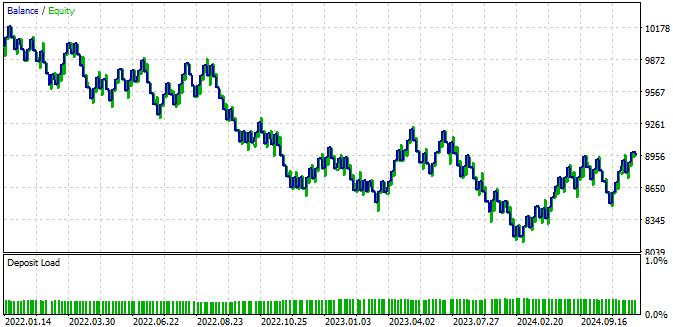
Fig 6: The equity curve produced by our current version of our trading strategy
When we analyze the detailed results of our trading strategy, we can observe that our algorithm lost in exceeding $1000 during our 3 years back test period. This is far from encouraging information. Additionally, our average and largest loss exceeds our average and largest profit. This gives us negative expectations of the strategy's performance in the future. Therefore, we would not want to use the strategy in its current form to trade an account with real capital.
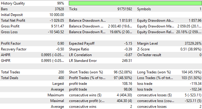
Fig 7: Analyzing the detailed results produced by our trading strategy
Improving on The Baseline
The foundation of our stop our prevention strategy, lies in an observation we made earlier in our series of discussions. Readers who may wish to revisit the prior discussion may find it readily available, here. In summary, we observed that over 200 different symbols on our MetaTrader 5 terminal, the moving average technical indicator appeared consistently easier to forecast, than price directly.
It is possible for us to put our observations to good use by forecasting if the future value of the moving average, is expected to surpass our stop loss level. If our computer expects that to be the case, then it should not place any trades for as long as it expects the moving average to hit our stop loss, otherwise our application will be allowed to place its trades.
This is the essence of our solution. It is clearly defined from start to finish, and is based on sound principles and objective reasoning. Let the reader note that we can even be more specific and require that in addition to not expecting our stop loss to be hit, our computer should also expect the moving average to surpass our take profit level, before taking any trade. Otherwise, why would anyone take a trade, if they don’t have reason to believe their take profit order will be filled?
To get us started, we first need to fetch the relevant market data from our MetaTrader 5 terminal, using an MQL5 script.
//+------------------------------------------------------------------+
//|                                                      ProjectName |
//|                                      Copyright 2020, CompanyName |
//|                                       http://www.companyname.net |
//+------------------------------------------------------------------+
#property copyright "Copyright 2024, MetaQuotes Ltd."
#property link      "https://www.mql5.com"
#property version   "1.00"
#property script_show_inputs

//--- Define our moving average indicator
#define MA_PERIOD 14                //--- Moving Average Period
#define MA_TYPE   MODE_EMA          //--- Type of moving average we have
#define MA_PRICE PRICE_CLOSE        //---- Applied Price of Moving Average

//--- Our handlers for our indicators
int ma_handle;

//--- Data structures to store the readings from our indicators
double ma_reading[];

//--- File name
string file_name = Symbol() + " Stop Out Prevention Market Data.csv";

//--- Amount of data requested
input int size = 3000;

//+------------------------------------------------------------------+
//| Our script execution                                             |
//+------------------------------------------------------------------+
void OnStart()
  {
//---Setup our technical indicators
   ma_handle = iMA(_Symbol,PERIOD_M30,MA_PERIOD,0,MA_TYPE,MA_PRICE);

//---Set the values as series
   CopyBuffer(ma_handle,0,0,size,ma_reading);
   ArraySetAsSeries(ma_reading,true);

//---Write to file
   int file_handle=FileOpen(file_name,FILE_WRITE|FILE_ANSI|FILE_CSV,",");

   for(int i=size;i>=1;i--)
     {
      if(i == size)
        {
         FileWrite(file_handle,"Time","Open","High","Low","Close","MA 14");
        }

      else
        {
         FileWrite(file_handle,
                   iTime(_Symbol,PERIOD_CURRENT,i),
                   iOpen(_Symbol,PERIOD_CURRENT,i),
                   iHigh(_Symbol,PERIOD_CURRENT,i),
                   iLow(_Symbol,PERIOD_CURRENT,i),
                   iClose(_Symbol,PERIOD_CURRENT,i),
                   ma_reading[i]);
        }
     }
//--- Close the file
   FileClose(file_handle);
  }
//+------------------------------------------------------------------+
Analyzing Our Data In Python
After you have applied the script onto your market of choice, we can begin analyzing our financial data using Python libraries. Our goal is to build a neural network, that can help us forecast the future value of the moving average indicator, and potentially keep us out of loosing trades.
import pandas as pd
import numpy as np
import seaborn as sns
import matplotlib.pyplot as plt
Now read in the data we extracted from our terminal.
data = pd.read_csv("EURUSD Stop Out Prevention Market Data.csv")
data
Label the data.
LOOK_AHEAD = 48
data['Target'] = data['MA 14'].shift(-LOOK_AHEAD)
data.dropna(inplace=True)
data.reset_index(drop=True,inplace=True)
Drop off the time periods that overlap with our back test.
#Let's entirely drop off the last 2 years of data
data.iloc[-((48 * 365 * 2) + (48 * 31 * 2) + (48 * 14) - (3)):,:]
Overwrite the original market data with the new data that doesn't contain the observations in our back test period.
#Let's entirely drop off the last 2 years of data
_ = data.iloc[-((48 * 365 * 2) + (48 * 31 * 2) + (48 * 14) - (3)):,:]
data = data.iloc[:-((48 * 365 * 2) + (48 * 31 * 2) + (48 * 14) - (3)),:]
data
Now load our machine learning libraries.
from sklearn.neural_network import MLPRegressor
from sklearn.model_selection import train_test_split,TimeSeriesSplit,cross_val_score
Create a time series split object so we can rapidly cross validate our model.
tscv = TimeSeriesSplit(n_splits=5,gap=LOOK_AHEAD)Specify the inputs and the target.
X = data.columns[1:-1]
y = data.columns[-1:]
Partition the data in half, for training and testing the new model.
train , test = train_test_split(data,test_size=0.5,shuffle=False)
Prepare the train and test partitions to be normalized and scaled.
train_X = train.loc[:,X]
train_y = train.loc[:,y]

test_X = test.loc[:,X]
test_y = test.loc[:,y]
Calculate the parameters for our z-scores.
mean_scores = train_X.mean()
std_scores = train_X.std()
Normalize the model's input data.
train_X = ((train_X - mean_scores) / std_scores)
test_X = ((test_X - mean_scores) / std_scores)
We want to perform a line search for the optimal number of training iterations for our deep neural network. We will iterate through increasing powers of 2. Starting from 2 to the power 0 until 2 to the power 14.
MAX_POWER = 15
results = pd.DataFrame(index=["Train","Test"],columns=[np.arange(0,MAX_POWER)])
Define a for loop that will help us estimate the optimal number of training iterations necessary to fit our deep neural network model onto the data we have.
#Classical Inputs
for i in np.arange(0,MAX_POWER):
    print(i)
    model = MLPRegressor(hidden_layer_sizes=(5,10,4,2),solver="adam",activation="relu",max_iter=(2**i),early_stopping=False)
    results.iloc[0,i] = np.mean(np.abs(cross_val_score(model,train_X.loc[:,:],train_y.values.ravel(),cv=tscv)))
    results.iloc[1,i] = np.mean(np.abs(cross_val_score(model,test_X.loc[:,:],test_y.values.ravel(),cv=tscv)))
    results
| 0 | 1 | 2 | 3 | 4 | 5 | 6 | 7 | 8 | 9 | 10 | 11 | 12 | 13 | 14 | |
|---|---|---|---|---|---|---|---|---|---|---|---|---|---|---|---|
| Train | 19675.492496 | 19765.297106 | 19609.7644 | 19511.588484 | 19859.734807 | 19942.30371 | 18831.617167 | 10703.554068 | 4930.771654 | 1639.952482 | 1389.615052 | 2938.371438 | 1.536765 | 2.193895 | 30.553918 |
| Test | 13171.519137 | 14113.252994 | 14428.159203 | 13649.157525 | 13655.643066 | 12919.773346 | 11472.770729 | 5878.964564 | 11293.444345 | 3788.388634 | 2545.368419 | 3599.364028 | 2240.598518 | 1041.641869 | 882.696622 |
Plotting the data visually shows that we need to take the maximum number of iterations to get the optimal output from our model. However, the reader should also be open-minded to the possibility that our search procedure may have terminated prematurely. Meaning that it is possible, we could've gotten better results if we used powers of 2 greater than 14. But, due to the computational cost of training these models, our search did not go past 2 to the power 14.
plt.title("Neural Network RMSE Forecasting 14 Period MA")
plt.ylabel("5 CV RMSE")
plt.xlabel("Training Iterations As Powers of 2")
plt.grid()
sns.lineplot(np.array(results.iloc[1,:]).transpose())
plt.axhline(results.min(1)[1],linestyle='--',color='red')
plt.axvline(14,linestyle='--',color='red')
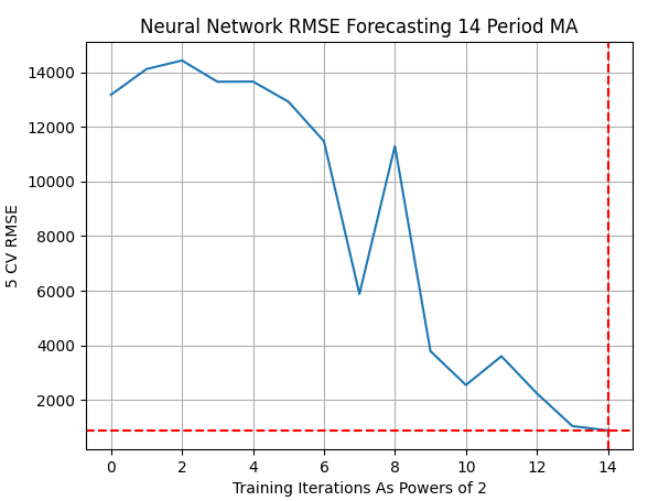
Fig 8: The results of searching for the optimal number of training iterations for our deep neural network model
Now that our model has been trained, we can now get ready to export our model to ONNX format.
import onnx
import skl2onnx
from skl2onnx.common.data_types import FloatTensorType
Prepare to fit the model using the optimal number of training iterations we have estimated.
model = MLPRegressor(hidden_layer_sizes=(5,10,4,2),solver="adam",activation="relu",max_iter=(2**14),early_stopping=False)
Load the z-scores for the entire dataset.
mean_scores = data.loc[:,X].mean()
std_scores = data.loc[:,X].std()

mean_scores.to_csv("EURUSD StopOut Mean.csv")
std_scores.to_csv("EURUSD StopOut Std.csv")
Transform the entire dataset.
data[X] = ((data.loc[:,X] - mean_scores) / std_scores)
Fit out model on all the data we have, excluding the test dates.
model.fit(data.loc[:,X],data.loc[:,'Target'].values.ravel())
Specify the input shape of our model.
initial_types = [("float_input",FloatTensorType([1,5]))]
Prepare to convert the model to ONNX format.
model_proto = skl2onnx.convert_sklearn(model,initial_types=initial_types,target_opset=12)Save the model as an ONNX file.
onnx.save(model_proto,"EURUSD StopOut Prevention Model.onnx")Building A Refined Version of Our Strategy
Let us begin building our new refined version of our trading strategy. First, load the ONNX model we have just finished creating.
//+------------------------------------------------------------------+
//|                                               Baseline Model.mq5 |
//|                                               Gamuchirai Ndawana |
//|                    https://www.mql5.com/en/users/gamuchiraindawa |
//+------------------------------------------------------------------+
#property copyright "Gamuchirai Ndawana"
#property link      "https://www.mql5.com/en/users/gamuchiraindawa"
#property version   "1.00"

//+------------------------------------------------------------------+
//| Resources                                                        |
//+------------------------------------------------------------------+
#resource "\\Files\\EURUSD StopOut Prevention Model.onnx" as uchar onnx_model_buffer[];
We shall create a few additional system constants for this version of our application.
//+------------------------------------------------------------------+
//| System constants                                                 |
//+------------------------------------------------------------------+
#define MA_PERIOD 14                 //--- Moving Average Period
#define MA_TYPE   MODE_EMA           //--- Type of moving average we have
#define MA_PRICE PRICE_CLOSE         //---- Applied Price of Moving Average
#define TF_1 PERIOD_D1               //--- Our time frame for technical analysis
#define TF_2 PERIOD_M30              //--- Our time frame for managing positions
#define VOL 0.1                      //--- Our trading volume
#define SL_SIZE  1e3 * _Point        //--- The size of our stop loss
#define SL_ADJUSTMENT 1e-5 * _Point  //--- The step size for our trailing stop
#define ONNX_MODEL_INPUTS 5          //---- Total model inputs for our ONNX model
Additionally, our global z-scores must be loaded into arrays.
//+------------------------------------------------------------------+
//| Our global variables                                             |
//+------------------------------------------------------------------+
int     ma_handler,system_state;
double  ma[];
double  mean_values[ONNX_MODEL_INPUTS]  = {1.157641086508574,1.1581085911361018,1.1571729541088953,1.1576420747040126,1.157640521193191};
double  std_values[ONNX_MODEL_INPUTS]   = {0.04070388112283021,0.040730761156963606,0.04067819202368064,0.040703752648947544,0.040684857239172416};
double  bid,ask,yesterday_high,yesterday_low;
const   string last_high = "LAST_HIGH";
const   string last_low  = "LAST_LOW";
long    onnx_model;
vectorf model_forecast = vectorf::Zeros(1);
Before we can use our ONNX models, we must first set the models accordingly and check if they have been correctly configured.
//+------------------------------------------------------------------+
//| Prepare the resources our EA requires                            |
//+------------------------------------------------------------------+
bool setup(void)
  {
   onnx_model = OnnxCreateFromBuffer(onnx_model_buffer,ONNX_DEFAULT);

   if(onnx_model == INVALID_HANDLE)
     {
      Comment("Failed to create ONNX model: ",GetLastError());
      return(false);
     }

   ulong input_shape[] = {1,ONNX_MODEL_INPUTS};
   ulong output_shape[] = {1,1};

   if(!OnnxSetInputShape(onnx_model,0,input_shape))
     {
      Comment("Failed to set ONNX model input shape: ",GetLastError());
      return(false);
     }

   if(!OnnxSetOutputShape(onnx_model,0,output_shape))
     {
      Comment("Failed to set ONNX model output shape: ",GetLastError());
      return(false);
     }

   ma_handler    = iMA(Symbol(),TF_2,MA_PERIOD,0,MA_TYPE,MA_PRICE);

   if(ma_handler == INVALID_HANDLE)
     {
      Comment("Failed to load technical indicator: ",GetLastError());
      return(false);
     }

   return(true);
  };
Our procedure for finding a trade setup is going to change slightly. We will first, fetch a prediction from our model. Afterward, our condition for opening and closing positions remain the same. However, in addition to these conditions being satisfied, we will also check for new conditions to be satisfied.
//+------------------------------------------------------------------+
//| Check if we have any trading setups                              |
//+------------------------------------------------------------------+
void find_setup(void)
  {
   if(!model_predict())
     {
      Comment("Failed to get a forecast from our model");
      return;
     }

   if((iHigh(Symbol(),TF_2,1) < yesterday_low) && (iHigh(Symbol(),TF_2,2) < yesterday_low))
     {
      if(iClose(Symbol(),TF_2,1) > ma[0])
        {
         check_buy();
        }
     }

   if((iLow(Symbol(),TF_2,1) > yesterday_high) && (iLow(Symbol(),TF_2,2) > yesterday_high))
     {
      if(iClose(Symbol(),TF_2,1) < ma[0])
        {
         check_sell();
        }
     }
  }
The new conditions we need to specify will apply to both our long and short positions. First, we will check to see if our forecast of the moving average is greater than the current reading of the moving average indicator that we have available. Additionally, we will also want to check if the future expected value of the moving average indicator, is greater than the current price reading being offered.
This means that our computer suspects the trend is likely to continue moving in one direction. Lastly, we will check whether our computer expects the moving average to remain beneath the stop loss. If all our conditions are satisfied, then we will open a position in the market right away.
//+------------------------------------------------------------------+
//| Check if we have a valid buy setup                               |
//+------------------------------------------------------------------+
void check_buy(void)
  {
   if((model_forecast[0] > ma[0]) && (model_forecast[0] > iClose(Symbol(),TF_2,0)))
     {
      if(model_forecast[0] > (bid - (SL_SIZE)))
         Trade.Buy(VOL,Symbol(),ask,(bid - (SL_SIZE)),(bid + (SL_SIZE)));
     }
  }
Our conditions for opening short positions will be the same as the conditions we specified for our long positions, but they will work in the opposite order.
//+------------------------------------------------------------------+
//| Check if we have a valid sell setup                              |
//+------------------------------------------------------------------+
void check_sell(void)
  {
   if((model_forecast[0] < ma[0]) && (model_forecast[0] < iClose(Symbol(),TF_2,0)))
     {
      if(model_forecast[0] < (ask + (SL_SIZE)))
         Trade.Sell(VOL,Symbol(),bid,(ask + (SL_SIZE)),(ask - (SL_SIZE)));
     }
  }
Once we have opened a position, we must continue to monitor it. Our update stop loss function will serve 2 purposes depending on how it is called. It takes a flag parameter that modifies its behavior. If the flag is set to 0, we are simply looking for an opportunity to push our stop levels towards more profitable prices. Otherwise, if the flag is set to 1, we want to first fetch a fresh forecast from our model and check if the future value of the moving average, may exceed our current stop loss level.
If the moving average is expected to surpass our stop loss but still form a profitable move, then we will adjust our stop loss to the level we expect the moving average to hit at its peak. Otherwise, if the trade is expected to fall beneath its opening price, then we want to instruct our computer to risk less on such trades, that show little potential for profit.
//+------------------------------------------------------------------+
//| Update our stop loss                                             |
//+------------------------------------------------------------------+
void update_sl(int flag)
  {
   //--- First find our open position
   if(PositionSelect(Symbol()))
     {
      double current_sl = PositionGetDouble(POSITION_SL);
      double current_tp = PositionGetDouble(POSITION_TP);
      double open_price = PositionGetDouble(POSITION_PRICE_OPEN);

      //--- Flag 0 means we just want to push the stop loss and take profit forward if its possible
      if(flag == 0)
        {
         //--- Buy Setup
         if(current_tp > current_sl)
           {
            if((bid - SL_SIZE) > current_sl)
               Trade.PositionModify(Symbol(),(bid - SL_SIZE),(bid + SL_SIZE));
           }

         //--- Sell setup
         if(current_tp < current_sl)
           {
            if((ask + SL_SIZE) < current_sl)
               Trade.PositionModify(Symbol(),(ask + SL_SIZE),(ask - SL_SIZE));
           }
        }

      //--- Flag 1 means we want to check if the stop loss may be hit soon, and act accordingly
      if(flag == 1)
        {
         model_predict();

         //--- Buy setup
         if(current_tp > current_sl)
           {

            if(model_forecast[0] < current_sl)
              {
               if((model_forecast[0] > ma[0]) && (model_forecast[0] > yesterday_low))
                  Trade.PositionModify(Symbol(),model_forecast[0],current_tp);
              }

            if(model_forecast[0] < open_price)
               Trade.PositionModify(Symbol(),model_forecast[0] * 1.5,current_tp);
           }

         //--- Sell setup
         if(current_tp < current_sl)
           {
            if(model_forecast[0] > current_sl)
              {
               if((model_forecast[0] < ma[0]) && (model_forecast[0] < yesterday_high))
                  Trade.PositionModify(Symbol(),model_forecast[0],current_tp);
              }

            if(model_forecast[0] > open_price)
               Trade.PositionModify(Symbol(),model_forecast[0] * 0.5,current_tp);
           }
        }
     }
  }
Our update procedure is modified slightly, to call the update stop loss function.
//+------------------------------------------------------------------+
//| Perform our update routines                                      |
//+------------------------------------------------------------------+
void update()
  {
//--- Daily procedures
     {
      static datetime time_stamp;
      datetime current_time = iTime(Symbol(),TF_1,0);
      if(time_stamp != current_time)
        {
         yesterday_high = iHigh(Symbol(),TF_1,1);
         yesterday_low = iLow(Symbol(),TF_1,1);
         //--- Mark yesterday's levels
         ObjectDelete(0,last_high);
         ObjectDelete(0,last_low);
         ObjectCreate(0,last_high,OBJ_HLINE,0,0,yesterday_high);
         ObjectCreate(0,last_low,OBJ_HLINE,0,0,yesterday_low);
        }
     }
//--- M30 procedures
     {
      static datetime time_stamp;
      datetime current_time = iTime(Symbol(),TF_2,0);
      if(time_stamp != current_time)
        {
         time_stamp = current_time;
         //--- Get updated prices
         bid = SymbolInfoDouble(Symbol(),SYMBOL_BID);
         ask = SymbolInfoDouble(Symbol(),SYMBOL_ASK);
         //--- Update our technical indicators
         CopyBuffer(ma_handler,0,0,1,ma);
         //--- Check for a setup
         if(PositionsTotal()==0)
            find_setup();

         //--- Check for a setup
         if(PositionsTotal() > 0)
            update_sl(1);
        }
     }
//--- Per tick procedures
     {
      //--- These function calls can become expensive and may slow down the speed of your back tests
      //--- Be thoughtful when placing any function calls in this scope
      update_sl(0);
     }
  }
We also need a dedicated function responsible for fetching predictions from our neural network model. We will first prepare the inputs into a float vector type, and then proceed to standardize the inputs, so we can fetch a prediction from our model.
//+------------------------------------------------------------------+
//| Get a forecast from our deep neural network                      |
//+------------------------------------------------------------------+
bool model_predict(void)
  {
   double ma_input[] = {0};
   CopyBuffer(ma_handler,0,1,1,ma_input);
   vectorf model_inputs =
     {
      (float) iOpen(Symbol(),TF_2,1),
      (float) iHigh(Symbol(),TF_2,1),
      (float) iLow(Symbol(),TF_2,1),
      (float) iClose(Symbol(),TF_2,1),
      (float) ma_input[0]
     };

   for(int i = 0; i < ONNX_MODEL_INPUTS;i++)
     {
      model_inputs[i] = (float)((model_inputs[i] - mean_values[i]) / std_values[i]);
     }

   if(!OnnxRun(onnx_model,ONNX_DEFAULT,model_inputs,model_forecast))
     {
      Comment("Failed to obtain forecast: ",GetLastError());
      return(false);
     }

   Comment(StringFormat("Expected MA Value: %f",model_forecast[0]));
   return(true);
  }
Lastly, when our application is no longer in use, we will release the indicator and the ONNX model.
//+------------------------------------------------------------------+
//| Free resources we are no longer using up                         |
//+------------------------------------------------------------------+
void release(void)
  {
   OnnxRelease(onnx_model);
   IndicatorRelease(ma_handler);
  }
//+------------------------------------------------------------------+
When we analyze the equity curve produced by our new refined version of our trading algorithm, we can quickly observe that the characteristic negative slope we observe in the first implementation of the strategy has been rectified, and our strategy now exhibits a positive trend, with occasional dips. This is more desirable than the initial state of our strategy.
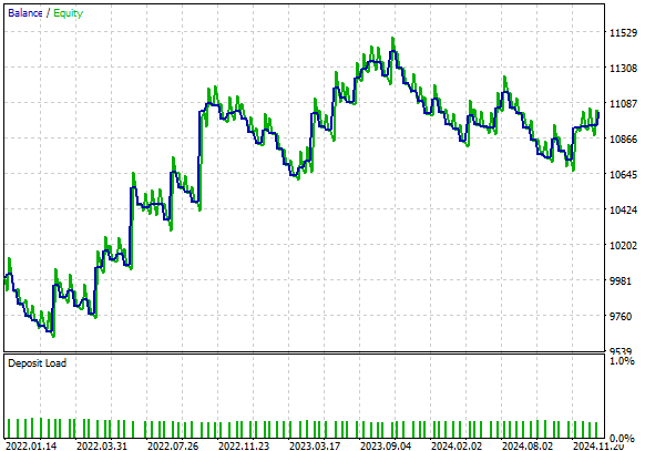
Fig 9: Visualizing the profit curve produced by our new refined version of our stop our prevention algorithm
Upon closer inspection, we find that our new strategy is now profitable. The initial version of our strategy, lost approximately $1000, and our current version has made slightly more than $1000. This is a major improvement. Our initial Sharpe ratio was -0.39 and our new Sharpe ratio is 0.79. The reader will also notice that our average profit trade grew from $98 to $130, while the average losing trade fell from $102 to $63. This shows that our average profits are growing at a significantly faster rate, than our average losses. These metrics give us positive expectations if we consider using this version of our trading strategy.
Although we have made significant progress, the problem of getting stopped out is certainly still a difficult problem to solve. This is evident to us by the fact that circa 60% of all the positions we opened, were losing trades. It is challenging to try to completely filter out all the trades that will get a trader stopped out, for today we managed to filter out most of the large and unprofitable trades.
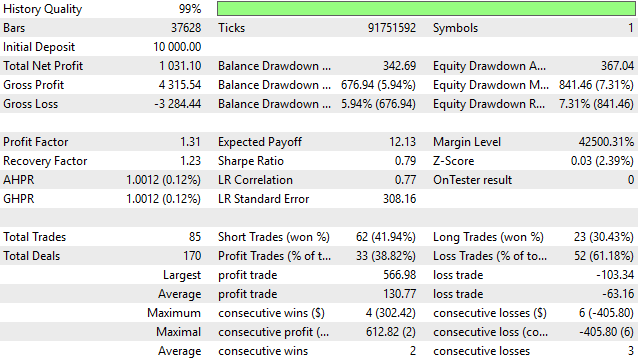
Fig 10: A detailed analysis of the results we obtained using our new stop out prevention algorithm
Conclusion
In this article, we have walked the reader through a potential solution to the long-standing problem of getting stopped out of winning trades. This problem lies at the heart of successful trading, and may never be completely solved. Each new solution introduces its own set of vulnerabilities into our strategy. After reading this article, the reader walks away with a more quantitative framework for managing their stop loss levels. Identifying and filtering out trades that will unnecessarily draw down your account, is a crucial component of any trading strategy.
| File Name | File Description |
|---|---|
| Baseline Model.mq5 | Our original trading strategy that we aimed to outperform. |
| Stop Out Prevention Model.mq5 | Our refined version of the trading strategy, powered by a deep neural network. |
| EURUSD Stop Out Moving Average Model.ipynb | The Jupyter Notebook we used to analyze the financial data we extracted from our MetaTrader 5 Terminal. |
| EURUSD Stop Out Prevention Model.onnx | Our Deep Neural Network. |
| Fetch Data MA.mq5 | The MQL5 script we used to fetch the requisite market data. |
- Free trading apps
- Over 8,000 signals for copying
- Economic news for exploring financial markets
You agree to website policy and terms of use