MQL5 Wizard Techniques you should know (Part 35): Support Vector Regression

Introduction

Support Vector Regression (SVR) is a form of regression derived from Support Vector Machines. At its core, SVR uses kernel methods to map input data into higher-dimensional spaces, allowing for more complex relationships to be captured, which contrasts with dimensionality reduction. For this article though we are exploring strictly its loss function role when used with a multi-layer perceptron. A related but different form of regression we looked at in an earlier article was Gaussian Process Regression. So perhaps it is key we start by drawing distinctions between the two.

Differences between SVR & GPR

To highlight the differences between these two, let us take a break from machine-learning-lingo and use everyday case examples to show why each is important. So, consider a scenario where you’re running a start-up that has developed a very healthy low sugar ice-cream that has a healthy demand in your hometown. Because you are just starting out and have only sold the ice cream in your home town you are still performing most of the manufacturing manually. You therefore need to start ramping up your productivity as this in addition to cost control, brings with it benefits like quality control, and implementing of some production standards.

Such an expansion, would require capital which you cannot borrow institutionally because you lack the necessary collateral (or wherewithal) to pitch to this to Banks; or you could partner with large established ice-cream brand however employees of large established brands are often bureaucrats and are going to say no regardless of what they think of your product.

So, you are left with the only option of raising capital via a private, semi-formal route and it comes with the caveat that you have to scale or expand your product. However, as you expand outside of you home town, which customers are going to look at or even consider your product vs the established brands? Being uncharted territory, you cannot approach it the same way you did home town. This then, does raise the question which you may have overlooked in your early hustle to meet home demand which is what is your primary customer segment?

Customer segmentation, a business aspect which some may choose to ignore, does have a number of types. It does include (but is not limited to) segment by zip-code (or address), segment by age, education level, occupation/ profession, and segment by income level; and another ‘new’ and growing segment thanks to social media could be segment lifestyle/ interest groups. By augmenting sales data by these segments, we can create a few interesting data sets that when gathered even over our home town, could provide a window into what happen next outside of our primary location.

Gaussian Process Regression, as introduced in an earlier article provides not just a mean projection, but it also attaches an indicative range to this mean together with a confidence level. This tends to mean it is suitable for making projections in situations where the demand for a product is hugely influenced by external factors (is not consistent) and is therefore a luxury or expensive product to make up for the inconsistent demand runs. If it’s not a luxury product then it could be highly seasonal or it could be a niche product with a high price point and fluctuating demand. This would mean our ice-cream would have to be at higher price point than the competition in order to fit the niche/ luxury product best suited for use with GPR.

In addition, the type of product and segmentation of the customer do present a confluence of choices when selecting a data set to project demand going forward which needs careful consideration as illustrated in the table below.

Segmentation Type	Best with SVR	Best with GPR
Zip Code	Everyday consumer goods	Not ideal unless combined with other dynamic data
Age	Apparel, consumer goods, educational tools	Not ideal unless combined with other dynamic data
Education Level	Educational products, tech products	Not ideal unless complex factors are at play
Income Level	Basic products in stable markets	Luxury goods, high-end electronics, premium items
Occupation	Products linked to stable occupations	Seasonal products, items influenced by external factors (e.g., weather)
Lifestyle/Interest Groups	Predictable interest groups (e.g., fitness apparel)	Specialty or niche products, highly variable demand

While our table above is not necessarily a factual portrayal of the relationship between customer segments and product types, it does emphasize the important point of considering these before selecting an appropriate data set to make forecasts. GPR to sum up, is better suited for businesses that often face uncertainty and complex growth patterns which necessitate the need to make predictions with confidence intervals.

Support Vector Regressions on the other hand are good for making projections where certainty and stable growth is in play. They are ideal for when decisions can be based on linear or moderately linear trends. Why? Because SVR is robust to noise. It focuses on getting the decision boundary that maximizes the margin of error while minimizing outlier influence. By having the error margin (epsilon) act as a classifier SVR should be effective with data sets that do not have a lot of outliers.

And as we can see from the cross-table recommendation above, SVR is best fitted in making projections for staples or everyday consumer goods for which demand is almost constant and barring a COVID-outbreak event (which can spike and crash demand) the level of demand for the product should not fluctuate a lot if at all. So, to consider our situation of expanding our ice cream sales outside of the hometown, SVR would be a suitable tool if it is not priced too ostensibly (as had been recommendation for GPR above) but is priced and shelved within stores at shelf-points where consumers pick up their daily groceries and staples they may need for the week.

So, if we use the cross table as a guide, if our ice-cream is a premium product that we sell mostly on major holidays, or only in the summer, or is offered to particular high-end restaurants, for example, then we are looking to use GVR with sales data that is aggregated by income level. In addition, the cross-table recommends consumer occupation and lifestyle / special interest groups and these too could be considered as well. On the flip side SVR would work best if our product was sold predominantly in big box stores where low-prices are important as argued above and the consumer segment to which this is pertinent is the address (or zip code). Aggregated sales data by address would therefore serve better in making projections with SVR on how fast or slow we should role out our ice-cream expansion as this is something we would have to get right since we are now using other-people’s money.

So, GVR serves best in forecasting situation where a high degree of uncertainty is acceptable while SVR, which we are focusing on for this article, is almost at the other end of the spectrum in that it ignores outliers that fall outside of a designated threshold when defining the data-sets’ hyper-plane.

SVR Definition

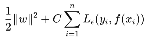
SVR can be formulated as an objective function and as a decision function. If we start with the formula to the objective function it is as follows:

Where

• w is the weight vector (parameters of the model) in our case we are interested in the L2-Norm of the weight matrices,
• C is the regularization parameter controlling the trade-off between model complexity and tolerance to mis-classification,
• L ϵ is the ϵ -insensitive loss function defined by:

Where

• f(xi ) is the predicted value,
• yi is the true value,
• ϵ defines a margin of tolerance within which no penalty is given for errors.

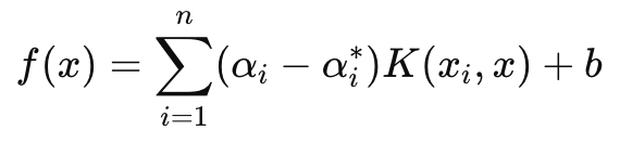
The decision function on the other hand that is chiefly used in forecasting, has the following formula:

Where

• αi and αi ^∗ are the Lagrange multipliers,
• K (xi , x) is the kernel function (e.g., linear, polynomial, RBF),
• b is the bias term.

As mentioned above SVR introduces a loss-insensitive parameter epsilon that sees to it that errors with a magnitude less than epsilon are ignored and do not result in weights or parameter adjustments for the model that is being trained. This makes SVR more robust to handling small noise and variations in data such that it can focus on the bigger picture or major trends.

In addition, in our objective function the C parameter manages the trade-off between minimizing the training error and minimizing the model’s complexity. A higher C minimizes the training error but risks over-fitting while a lower C, on paper, would lead to more generalization and better flexibility when making forecasts in different scenarios.

We are strictly going to focus on using the loss function of SVR when training a simple MLP for this network. We will not make projections with its kernels as would be the case with the decision function. However, it is worth mentioning that SVR uses kernel functions to transform input data into a higher-dimensional space where relationships that may not be linear in the original space can be pin-pointed. Common kernels for this include: the linear kernel, polynomial kernel and the RBF.

SVR loss function can be implemented in MQL5 as follows:

//+------------------------------------------------------------------+
//| SVR Loss                                                         |
//+------------------------------------------------------------------+
vector Cmlp::SVR_Loss()
{  vector _loss = fabs(output - label);
   for(int i = 0; i < int(_loss.Size()); i++)
   {  if(_loss[i] <= THIS.svr_epsilon)
      {  _loss[i] = 0.0;
      }
   }
   vector _l = THIS.svr_c*_loss;
   double _w = 0.5 * WeightsNorm(MATRIX_NORM_P2);
   vector _weight_norms;
   _weight_norms.Init(_loss.Size());
   _weight_norms.Fill(_w);
   return(_weight_norms + _l);
}

Typically, this loss value is a scalar, however because this loss function is now being used in back propagation and certain networks have more than one final output, it was important to maintain the loss structure in a vector form even though SVR condenses this to a scalar. And that is what we have done. Also, within the backpropagation function, we check and see if the SVR loss is being used. This is as indicated below:

//+------------------------------------------------------------------+
//| BACKWARD PROPAGATION OF THE MULTI-LAYER-PERCEPTRON.              |
//+------------------------------------------------------------------+
//|                                                                  |
//| -Extra Validation check of MLP architecture settings is performed|
//|  at run-time.                                                    |
//|  Chcecking of 'validation' parameter should ideally be performed |
//|  at class instance initialisation.                               |
//|                                                                  |
//| -Run-time Validation of learning rate, decay rates and epoch     |
//|  index is performed as these are optimisable inputs.             |
//+------------------------------------------------------------------+
void Cmlp::Backward(Slearning &Learning, int EpochIndex = 1)
{  if(!validated)
   {  printf(__FUNCSIG__ + " invalid network arch! ");
      return;
   }
   
   ...


   if(EpochIndex < 0)
   {  printf(__FUNCSIG__ + " Epoch Index Should start from 1. ");
      return;
   }


    ...


   vector _last_loss = (THIS.svr_loss? SVR_Loss():output.LossGradient(label, THIS.loss));

    ....
}

We are able to add this one-line modification because our constructor parameters are in a struct and we easily modified this struct, (since this class was introduced in earlier articles) as follows:

//+------------------------------------------------------------------+
//| Multi-Layer-Perceptron Struct for Constructor Parameters         |
//+------------------------------------------------------------------+
struct Smlp
{  //arch array must be defined with at least 2 non zero values
   //that represent the size of the input layer and output layer
   //If more values than this are provided in the array then the
   //middle values will define the size(s) of the hidden layer(s)
   //first value (index zero) is size of input layer
   //last value (index size-1) is size of output layer
   int               arch[];


  ...


   bool              svr_loss;
   double            svr_c;
   double            svr_epsilon;

                     Smlp()
   {                 ArrayFree(arch);

     ...

      svr_loss = false;
      svr_c = 1.0;
      svr_epsilon = __EPSILON * 5.0;
   };
                    ~Smlp() {};
};

Implementing a Signal Class

To have a signal class with an MLP whose loss function uses the SVR, we would be using our already coded class for an MLP that was shared in previous articles. The changes necessary to this class for us to use the SVR loss are already highlighted above so what is left is how this class is called and used within a custom instance of a signal class. Our MLP’s covered recently in these series are all trying to forecast the next change in close price on each new bar. This means on a timer basis (each new bar) fresh computations are made for what the next change in close price will be.

The inputs for calculating this are also prior close price changes with the main variable in this being the number of these changes. (This variable establishes the input layer size). Alternatives are possible in defining not just what inputs should be fed into the MLP when projecting the next bar close price change but also on how forward looking the forecast should be. The last point is important because for our testing purposes we are using a single price bar forward outlook. In addition, prior to making each forecast, we do perform a back propagation on each new bar to train our network over a given training set size for an input defined number of epochs.

These two input parameters ‘training set size’, and ‘epochs’ are also optimizable and this calls for a balance between getting the ideal weights of the network and generalization. This is because while a larger training set and more epochs can indicate a good performance on the sampled data, a cross validation is bound to not be as rosy unless the network has some generalization and is not overly fit to its training data. The Get Output function handles the forecasting through the MLP and its source code is shared below:

//+------------------------------------------------------------------+
//|                                                                  |
//+------------------------------------------------------------------+
void CSignalSVR::GetOutput(vector &Output)
{  m_learning.rate = m_learning_rate;
   for(int i = m_epochs; i >= 1; i--)
   {  MLP.LearningType(m_learning, i);
      for(int ii = m_train_set; ii >= 0; ii--)
      {  vector _in, _in_new, _in_old;
         if
         (
            _in_new.Init(__MLP_SIGN_INPUTS) &&
            _in_new.CopyRates(m_symbol.Name(), m_period, 8, ii + __MLP_SIGN_OUTPUTS, __MLP_SIGN_INPUTS) &&
            _in_new.Size() == __MLP_SIGN_INPUTS &&
            _in_old.Init(__MLP_SIGN_INPUTS) &&
            _in_old.CopyRates(m_symbol.Name(), m_period, 8, ii + __MLP_SIGN_OUTPUTS + __MLP_SIGN_OUTPUTS, __MLP_SIGN_INPUTS) &&
            _in_old.Size() == __MLP_SIGN_INPUTS
         )
         {  _in = _in_new - _in_old;
            MLP.Set(_in);
            MLP.Forward();
            if(ii > 0)
            {  vector _target, _target_new, _target_old;
               if
               (
                  _target_new.Init(__MLP_SIGN_OUTPUTS) &&
                  _target_new.CopyRates(m_symbol.Name(), m_period, 8, ii, __MLP_SIGN_OUTPUTS) &&
                  _target_new.Size() == __MLP_SIGN_OUTPUTS &&
                  _target_old.Init(__MLP_SIGN_OUTPUTS) &&
                  _target_old.CopyRates(m_symbol.Name(), m_period, 8, ii + __MLP_SIGN_OUTPUTS, __MLP_SIGN_OUTPUTS) &&
                  _target_old.Size() == __MLP_SIGN_OUTPUTS
               )
               {  _target = _target_new - _target_old;
                  MLP.Get(_target);
                  MLP.Backward(m_learning, i);
               }
            }
            Output = MLP.output;
         }
      }
   }
}

It does not differ significantly from implementations we have had in prior articles. The backpropagation is performed for each training set data point that has a label (or target value). Usually, all training data has a target value but because in our case we are merging with forecasting, the final ‘training data point’ is current and its eventual close price change is what we are seeking. So, when we get to the current input data that are supposed to give us our forecast, we do not perform any training. Also, this is why we are counting down in each training set i.e. we first train with very old data and then work our way downwards to the current data.

Implementing a Trailing Stop Class

It has been awhile in these series since we considered anything other than a custom signal class and yet readers who saw my earlier articles will recall that I often shared trade ideas not just as a signal class but also trailing stop classes and even money management classes. So, we return to these straits by considering a custom trailing stop class that can be attached to an Expert Advisor via the MQL5 wizard. Guidance, for new readers, on how the code that is shared below can be used in the MQL5 wizard to create an Expert Advisor can be found here and here.

So, to implement a custom trailing class, we will be looking to check if for any open position that either does not have a stop loss and needs one to be introduced or one that already has a stop loss but needs it to be adjusted to better lock in profits. Stop losses are a little bit controversial because they are never guaranteed. Only limit order prices are. If for whatever reason, the market moves more than most people anticipated then the broker will only be able to close your order at the next ‘available price’, not your stop loss. This notwithstanding, we are going to make the decision to set or move the stop loss based on the forecast magnitude change in price-bar range. We implement this in another Get Output function, similar but different to what we had with the custom signal class. This is shared below:

//+------------------------------------------------------------------+
//|                                                                  |
//+------------------------------------------------------------------+
void CTrailingSVR::GetOutput(vector &Output)
{  m_learning.rate = m_learning_rate;
   for(int i = m_epochs; i >= 1; i--)
   {  MLP.LearningType(m_learning, i);
      for(int ii = m_train_set; ii >= 0; ii--)
      {  vector _in, _in_new_hi, _in_new_lo, _in_old_hi, _in_old_lo;
         if
         (
            _in_new_hi.Init(__MLP_TRAIL_INPUTS) &&
            _in_new_hi.CopyRates(m_symbol.Name(), m_period, 2, ii + __MLP_TRAIL_OUTPUTS, __MLP_TRAIL_INPUTS) &&
            _in_new_hi.Size() == __MLP_TRAIL_INPUTS &&
            _in_old_hi.Init(__MLP_TRAIL_INPUTS) &&
            _in_old_hi.CopyRates(m_symbol.Name(), m_period, 2, ii + __MLP_TRAIL_OUTPUTS + __MLP_TRAIL_OUTPUTS, __MLP_TRAIL_INPUTS) &&
            _in_old_hi.Size() == __MLP_TRAIL_INPUTS
            &&
            _in_new_lo.Init(__MLP_TRAIL_INPUTS) &&
            _in_new_lo.CopyRates(m_symbol.Name(), m_period, 4, ii + __MLP_TRAIL_OUTPUTS, __MLP_TRAIL_INPUTS) &&
            _in_new_lo.Size() == __MLP_TRAIL_INPUTS &&
            _in_old_lo.Init(__MLP_TRAIL_INPUTS) &&
            _in_old_lo.CopyRates(m_symbol.Name(), m_period, 4, ii + __MLP_TRAIL_OUTPUTS + __MLP_TRAIL_OUTPUTS, __MLP_TRAIL_INPUTS) &&
            _in_old_lo.Size() == __MLP_TRAIL_INPUTS
         )
         {  vector _in_new = _in_new_hi - _in_new_lo;
            vector _in_old = _in_old_hi - _in_old_lo;
            _in = _in_new - _in_old;
            MLP.Set(_in);
            MLP.Forward();
            if(ii > 0)
            {  vector _target, _target_new_hi, _target_old_hi, _target_new_lo, _target_old_lo;
               if
               (
                  _target_new_hi.Init(__MLP_TRAIL_OUTPUTS) &&
                  _target_new_hi.CopyRates(m_symbol.Name(), m_period, 8, ii, __MLP_TRAIL_OUTPUTS) &&
                  _target_new_hi.Size() == __MLP_TRAIL_OUTPUTS &&
                  _target_old_hi.Init(__MLP_TRAIL_OUTPUTS) &&
                  _target_old_hi.CopyRates(m_symbol.Name(), m_period, 8, ii + __MLP_TRAIL_OUTPUTS, __MLP_TRAIL_OUTPUTS) &&
                  _target_old_hi.Size() == __MLP_TRAIL_OUTPUTS
                  &&
                  _target_new_lo.Init(__MLP_TRAIL_OUTPUTS) &&
                  _target_new_lo.CopyRates(m_symbol.Name(), m_period, 8, ii, __MLP_TRAIL_OUTPUTS) &&
                  _target_new_lo.Size() == __MLP_TRAIL_OUTPUTS &&
                  _target_old_lo.Init(__MLP_TRAIL_OUTPUTS) &&
                  _target_old_lo.CopyRates(m_symbol.Name(), m_period, 8, ii + __MLP_TRAIL_OUTPUTS, __MLP_TRAIL_OUTPUTS) &&
                  _target_old_lo.Size() == __MLP_TRAIL_OUTPUTS
               )
               {  vector _target_new = _target_new_hi - _target_new_lo;
                  vector _target_old = _target_old_hi - _target_old_lo;
                  _target = _target_new - _target_old;
                  MLP.Get(_target);
                  MLP.Backward(m_learning, i);
               }
            }
            Output = MLP.output;
         }
      }
   }
}

Our code above though almost identical to what we had in the signal is different mainly from the type of input data it receives and its expected output. We are trying to determine whether we need to move our stop loss and our prerequisite assumption for this is an uptick in volatility. Therefore, we need to find out what the next change in price bar range change is going to be. This sort of data is bound to be very volatile itself (or noisy) which is why if we had used moving average buffers as our input data and target values it could have been more prudent. This can be modified since full source is attached below, however, we are using changes in the highs minus lows of each price bar as inputs and we are looking for output to be the next change in these input values just like we had with close prices for the signal above.

So, if the projected change in price bar range is positive, implying volatility is increasing, we make steps to move our stop loss in proportion to our projected increase. This might seem foolhardy because as mentioned above broker’s never guarantee a stop loss price which is why the counter option of only moving a stop loss on projected decrease in volatility could be ‘more certain’ since in less volatile times brokers ae more likely to honor stop losses than when there is volatility. Yes, so it’s a bit of a debate and I leave this to the reader to explore and make appropriate adjustments to the code depending on his findings.

Strategy Tester Results

We perform testing on the pair USDJPY, on the daily time frame from 2023.01.01 to 2024.01.01. These test runs are performed with some of the best settings got from very quick and optimizations for which no forward walks or cross validation has been done. They are exhibited here to simply demonstrate ability to place trades and use the wizard assembled Expert Advisor. The extra diligence in testing over extended periods of history while also doing forward walks if optimization is involved is left up to the reader. It is noteworthy as well that wizard assembled Expert Advisors can combine multiple signals when developing a trading system so the testing or optimization does not have to be with the custom signals used here alone.

We have developed a custom signal with SVR and a custom trailing class with a similar MLP. The test runs presented below are therefore for two Expert Advisors whose interface code is attached below. The first uses only the custom signal with no trailing stop. Its results are presented below:

The second uses the custom signal and the custom trailing class we implemented above. Its results are also shown below.

Conclusion

To conclude, we have looked at Support Vector Regression, that follows another form of regression we considered when we looked at Gaussian Process Kernels. These two regressions, Support Vector Regression and Gaussian Process Regression are almost polar opposites in their application since SVR tends to be more suitable for less volatile and trending data sets while GPR thrives in more volatile and less certain environments. Support Vector Regression does feature an objective function and a decision function. We have sought to exploit the former, the objective function, as a loss function to a multi-layer perceptron in a signal class and a custom trailing stop class.

The use of the decision function, to act as a forecaster, would require the additional use of kernels, something we explored in the article on Gaussian Process Kernels, but have refrained from in this article since our forecaster was purely an MLP. In a future article(s) we could consider this given that there are different forms of kernels that can be used in performing this however the SVR loss function was our target for this article. By using a loss-insensitive parameter epsilon, it too, together with a growing list of loss function implementations some of which we covered here, can introduce a different way of training neural networks.

This loss-insensitive parameter epsilon acts more like a classifier than a regressor and one could argue that this makes the case for this loss function to be used more in classifier networks than regressor networks as we have done for this article and that could be true. However, SVR still deals with continuous outputs (decimal data sets) and predicts numerical values in a similar format. It simply uses the epsilon margin to decide whether an error should be penalized, but its goal remains regression, and not classification.