Gain An Edge Over Any Market (Part V): FRED EURUSD Alternative Data

MetaTrader 5 — Examples | 30 September 2024, 14:36

574

In this series of articles, our goal is to help you navigate the ever-growing landscape of alternative financial data. The modern investor, living in the age of big-data, may not possess enough resources to carefully decide which alternative data-sets he should include in his trading process. We aim to furnish you with the information you need, to arrive at an informed decision on which alternative datasets you should probably consider and which ones you may be better off without.

Overview of The Trading Strategy

Correlation is a cornerstone principle of an analytical approach to finance. If two assets are correlated, then investors who seek to either diversify their portfolios or maximize their exposure to anticipated price changes, may intelligently use this metric to build their portfolio.

The Federal Reserve System maintains a collection of indexes that serve as summary measures of the Foreign Exchange value of the Dollar. From all the indexes we had available, we were particularly interested in the Nominal Broad Dollar Daily Index (NBDD). The index was established in Jan 2006 with a value of 100 points. At the time of writing, the index set record lows of approximately 86 points during the 2008 recession and set its all-time high of roughly 128 points in 2022. The index has been in a bullish trend since late 2011 and is currently hovering around 121 points. This is well within the vicinity of its all-time high.

In the graph below, we have overlaid the Broad Dollar index and the EURUSD pair exchange rate. It is almost impossible to see any material relationship between the two time-series data. The US Dollar Exchange Rate is almost hidden as the flat line at the bottom of the graph in blue, while the Broad Dollar Index is the clearly visible red line.

FRED Data unscaled

Fig 1: The Dollars to Euro Spot Exchange Rate & the Broad Dollar Index

If we were to ensure that both time-series data are on the same scale, an obvious pattern emerges. We shall change our y-axis so that it records the percent change in time-series data over 1 year. When we perform this step, we can clearly observe that the index displays almost perfect negative correlation to the EURUSD Foreign Exchange rate.

FRED EURUSD Data

Fig 2: The Dollars to Euro Spot Exchange Rate & the Broad Dollar Index on a percentage scale

We shall explore the viability of algorithmically learning a trading strategy that employs these datasets to predict the future exchange rate of the EURUSD. Given the perfect negative correlation, there could potentially be some information that our model could learn about the exchange rate, given macroeconomic indicators from the Federal Reserve Economic Database (FRED).

Overview of The Methodology

To test the validity of our proposition, we started by fetching Daily historical exchange rates on the EURUSD from our MetaTrader 5 terminal, and merged the data with 3 macroeconomic datasets we retrieved from the FRED Python API. The 3 FRED time-series data-sets were recording:

Interest Rates on American Bonds
Expected Inflation Rates in the USA
Broad Dollar Index

This allowed us to create 3 datasets for building our AI model:

Ordinary OHLC market quotes.
Alternative FRED data
A superset of the first 2.

After merging all the datasets in question, and converting the scales to replicate what we did on the FRED website, we observed correlation levels between the prices of the EURUSD exchange rate and the Broad Dollar Index were almost -0.9. That is an almost perfect score! Not only that, but we also observed the correlation between the current value of the Broad Dollar Index and the future value, 20 days into the future, of the EURUSD close was -0.7.

Upon visualization, we were able to separate the time-series data remarkably well, with a level of finesse that I doubt we have demonstrated before in this series of articles. It appears that using the percent change in the data over relatively longer windows allows us to separate the data extremely well. Our 3D scatter-plots further validated how well the data was separated, and we could identify apparent bullish and bearish zones. Furthermore, when we performed scatter-plots of the data on the official FRED website, we could clearly observe a trend in the data. The trend in the scatter-plot was well-defined, even without having to use our usual bag of advanced analytical tools in Python. This gave us confidence that there could be some potential information being shared by the two time-series data sets that hopefully our model can learn.

FRED Data Has A Trend

Fig 3: Visualizing a scatter plot of the 2 datasets we are interested in

As promising as all of this may sound so far, none of this translated into improved performance in our ability to predict the future value of the EURUSD exchange rate. As a matter of fact, our performance only got worse, and it appears we were better off using the first dataset that only contained ordinary market quotes.

We trained 3 identical Deep Neural Network (DNN) Regressors to learn the relationship, between our 3 datasets and the common target they all shared. The first DNN model produced the lowest error rate. Moreover, none of our feature selection algorithms appeared impressed by any of the FRED Datasets we selected for our analysis. Not to be deterred, we successfully managed to tune our DNN model parameters using the training dataset, without overfitting to the training data. This is suggested to us by the fact that we outperformed the default DNN model on unseen validation data. We employed time-series cross validation without random shuffling to arrive at these decisions in training and validation.

Before we exported our model to ONNX format, we inspected the residuals of our model to ensure that our model is in sound condition. Unfortunately, the residuals we observed from our model were badly misbehaved, which may suggest that our model has failed to learn effectively.

Finally, we exported our model to ONNX format and built an integrated AI-powered expert advisor using Python and MQL5.

Fetching The Data

To get started, we first imported the Python libraries that we need.

#Import the libraries we need
from   fredapi           import Fred
import seaborn           as sns
import numpy             as np
import pandas            as pd
import MetaTrader5       as mt5
import matplotlib.pyplot as plt

Then we defined our credentials and which time-series we would like to fetch from FRED.

#Define important variables
fred_api                = "ENTER YOUR API KEY"
fred_broad_dollar_index = "DTWEXBGS"
fred_us_10y             = "DGS10"
fred_us_5y_inflation    = "T5YIFR"

#Login to fred
fred = Fred(api_key=fred_api)

Let us get the data we need.

#Fetch the data
dollar_index    = fred.get_series(fred_broad_dollar_index)
us_10y          = fred.get_series(fred_us_10y)
us_5y_inflation = fred.get_series(fred_us_5y_inflation)

Naming the series will allow us to merge them later on.

#Name the series so we can merge the data
dollar_index.name    =  "Dollar Index"
us_10y.name          =  "Bond Interest"
us_5y_inflation.name =  "Inflation"

Fill in any missing values with the rolling average.

#Fill in any missing values
dollar_index.fillna(dollar_index.rolling(window=5,min_periods=1).mean(),inplace=True)
us_10y.fillna(us_10y.rolling(window=5,min_periods=1).mean(),inplace=True)
us_5y_inflation.fillna(dollar_index.rolling(window=5,min_periods=1).mean(),inplace=True)

Before we can fetch data from our MetaTrader 5 terminal, we first need to initialize it.

#Initialize the terminal
mt5.initialize()

True

We would like to fetch 4 years of historical data.

#Define how much data to fetch
amount = 365 * 4
#Fetch data
eur_usd = pd.DataFrame(mt5.copy_rates_from_pos("EURUSD",mt5.TIMEFRAME_D1,0,amount))
eur_usd

Convert the time column from seconds format to actual dates.

#Convert the time column
eur_usd['time'] = pd.to_datetime(eur_usd.loc[:,'time'],unit='s')

Make sure the time column is the index of our data.

#Set the column as the index
eur_usd.set_index('time',inplace=True)

Define how far into the future we would like to forecast.

#Define the forecast horizon
look_ahead = 20

Let us now specify our predictors and targets.

#Define the predictors
predictors = ["open","high","low","close","tick_volume","Dollar Index","Bond Interest","Inflation"]
ohlc_predictors = ["open","high","low","close","tick_volume"]
fred_predictors = ["Dollar Index","Bond Interest","Inflation"]
target = "Target"
all_data = ["Target","open","high","low","close","tick_volume","Dollar Index","Bond Interest","Inflation"]
all_data_binary = ["Binary Target","open","high","low","close","tick_volume","Dollar Index","Bond Interest","Inflation"]

Merge the data.

#Merge our data
merged_data = eur_usd.merge(dollar_index,right_index=True,left_index=True)
merged_data = merged_data.merge(us_10y,right_index=True,left_index=True)
merged_data = merged_data.merge(us_5y_inflation,right_index=True,left_index=True)

Label the data.

#Define the target
target         = merged_data.loc[:,"close"].shift(-look_ahead)
target.name    =  "Target"

Format the data so that it shows us the annual percent change, just like the data we analyzed on the FRED website.

#Convert the data to yearly percent changes
merged_data = merged_data.loc[:,predictors].pct_change(periods = 365) * 100
merged_data = merged_data.merge(target,right_index=True,left_index=True)
merged_data.dropna(inplace=True)
merged_data

Add a binary target for plotting purposes.

#Add binary targets for plotting purposes
merged_data["Binary Target"] = 0
merged_data.loc[merged_data["close"] < merged_data["Target"],"Binary Target"] = 1

Reset the index of the data.

#Reset the index
merged_data.reset_index(inplace=True,drop=True)
merged_data

Exploratory Data Analysis

We shall start by recreating the plot we generated on the St. Louis Federal Reserve website, this will validate that we have performed our preprocessing steps as intended.

#Plotting our data set
plt.title("EURUSD Close Against FRED Broad Dollar Index")
plt.plot(merged_data.loc[:,"close"])
plt.plot(merged_data.loc[:,"Dollar Index"])

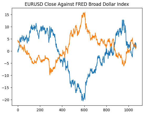
Fig 4: Recreating our observation on the FRED website in Python

Let us now analyze the correlation levels within our data-set. As we can observe, the inflation dataset has the weakest correlation levels from all 3 alternative FRED data-sets we have fetched. However, we did not gain any performance improvements even though our remaining 2 alternative data-sets appeared to have so much potential.

#Exploratory data analysis
sns.heatmap(merged_data.loc[:,all_data].corr(),annot=True)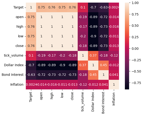

Fig 5: Our correlation heat-map

When viewing a lot of data-sets at once, pair plots can help us quickly see the relationships that may exist between all the data we have available. We can clearly see that the orange and blue dots appear to be remarkably well separated. Moreover, we have kernel-density estimation (kde) plots running along the main diagonal of this plot. KDE plots help us visualize the distribution of data within each column. The fact that we observe what appears to be 2 hills like shapes that overlap over a small section, implies that the data is for the most part well separated.

sns.pairplot(merged_data.loc[:,all_data_binary],hue="Binary Target")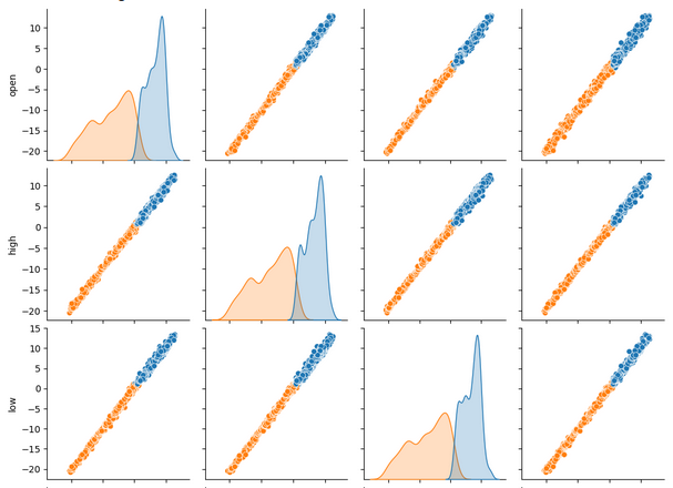

Fig 6: Visualizing our data using pair-plots

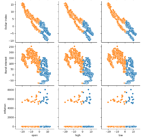
Fig 7: Visualizing our FRED alternative data and its relationship with our EURUSD pair

We shall now perform 3D scatter plots using the Broad Dollar Index and the Bond Interest Rate on the x and y-axis, and the EURUSD close on the z axis. The data appears to be in 2 distinct clusters, with little overlap. This would naturally imply that there could be a decision boundary our model could learn from the data. Regrettably, I believe we failed to expose this effectively to our model.

#Define the 3D Plot
fig = plt.figure(figsize=(7,7))
ax = plt.axes(projection="3d")
ax.scatter(merged_data["Dollar Index"],merged_data["Bond Interest"],merged_data["close"],c=merged_data["Binary Target"])
ax.set_xlabel("Dollar Index")
ax.set_ylabel("Bond Interest")
ax.set_zlabel("EURUSD close")

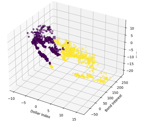
Fig 8: Visualizing our market data in 3D

Preparing To Model The Data

Let us now get ready to model the financial data we have, we shall start by defining our model inputs and target.

#Let's define our set of predictors
X = merged_data.loc[:,predictors]
y = merged_data.loc[:,"Target"]

Importing the library we need.

#Import the libraries we need
from sklearn.model_selection import train_test_split

Now we shall partition our data into the 3 groups we outlined earlier.

#Partition the data
ohlc_train_X,ohlc_test_X,train_y,test_y = train_test_split(X.loc[:,ohlc_predictors],y,test_size=0.5,shuffle=False)
fred_train_X,fred_test_X,_,_            = train_test_split(X.loc[:,fred_predictors],y,test_size=0.5,shuffle=False)
train_X,test_X,_,_                      = train_test_split(X.loc[:,predictors],y,test_size=0.5,shuffle=False)

Create a data-frame to store our model's cross-validation accuracy.

#Prepare the dataframe to store our validation error
validation_error = pd.DataFrame(columns=["MT5 Data","FRED Data","ALL Data"],index=np.arange(0,5))

Modelling The Data

Let us import the libraries we need to model the data.

#Let's cross validate our models
from sklearn.neural_network import MLPRegressor
from sklearn.model_selection import cross_val_score

Define the 3 neural networks we outlined earlier.

#Define the neural networks
ohlc_nn = MLPRegressor(hidden_layer_sizes=(10,20,40),max_iter=500)
fred_nn = MLPRegressor(hidden_layer_sizes=(10,20,40),max_iter=500)
all_nn  = MLPRegressor(hidden_layer_sizes=(10,20,40),max_iter=500)

Test each model.

#Let's obtain our cv score
ohlc_score = cross_val_score(ohlc_nn,ohlc_train_X,train_y,scoring='neg_root_mean_squared_error',cv=5,n_jobs=-1)
fred_score = cross_val_score(fred_nn,fred_train_X,train_y,scoring='neg_root_mean_squared_error',cv=5,n_jobs=-1)
all_score = cross_val_score(all_nn,train_X,train_y,scoring='neg_root_mean_squared_error',cv=5,n_jobs=-1)

Store our cross-validation scores.

for i in np.arange(0,5):
    validation_error.iloc[i,0] = ohlc_score[i]
    validation_error.iloc[i,1] = fred_score[i]
    validation_error.iloc[i,2] = all_score[i]

Visualize the validation error.

#Our validation error
validation_error

MetaTrader 5 Data	FRED Alternative Data	All Data
-0.147973	-0.79131	-4.816608
-0.103913	-2.073764	-0.655701
-0.211833	-0.276794	-0.838832
-0.094998	-1.954753	-0.259959
-1.233912	-2.152471	-3.677273

Analyzing our mean performance across all 5 folds shows that our ordinary market data from MetaTrader 5 may be our best bet.

#Our mean performane across all groups
validation_error.mean()

Input Data	Average 5-Fold Error
MetaTrader 5	-0.358526
FRED	-1.449818
ALL	-2.049675

When we plot the performance of our models, we can observe that the MetaTrader 5 data produced more consistent error levels.

#Plotting our performance
validation_error.plot()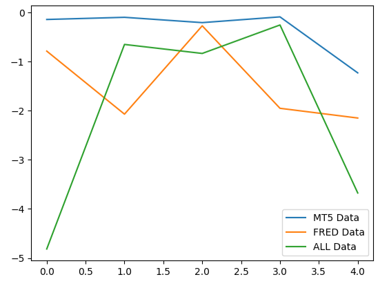

Fig 9: Visualizing the 3 different error levels produced by the 3 data-sets we had to choose from

The squashed shape of the MetaTrader 5 error box-plot is desirable because it shows that the model is demonstrating skill through its consistent performance.

#Creating box-plots of our performance
sns.boxplot(validation_error)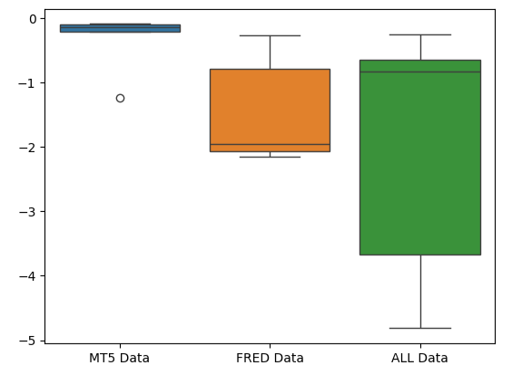

Fig 10: Visualizing our model's error metrics as box-plots

Feature Importance

Let us reason out which features may be most important to our DNN model. Hopefully, the alternative data we have selected is useful, then it shall be deemed so by our feature importance algorithms. Unfortunately, our analysis suggests that the variation in the MetaTrader 5 market data appears to explain the target reasonably well alone. Therefore, there was no additional information contained within the FRED time-series that our model could not have reasoned out from the data it had.

To get started, let us import the libraries we need.

#Feature importance
from alibi.explainers import ALE, plot_ale

Accumulated Local Effects (ALE) plots help us visualize the effect each model input has on the target. ALE Plots are popular for their robust capability to explain models that have been trained on data that is highly correlated, such as ours. Classical academic methods such as Partial Dependency (PD) plots, simply were not reliable when explaining predictors with strong correlation levels. The original specification of the algorithm can be read in the complete 2016 research paper by Daniel W. Apley and Jingyu Zhu linked, here.

Fig 11: Daniel W. Apley co-creator of the ALE algorithm

Let us fit the ale explainer to our DNN Regressor.

#Explaining our deep neural network
model = MLPRegressor(hidden_layer_sizes=(10,20,40),max_iter=500)
model.fit(train_X,train_y)
dnn_ale = ALE(model.predict,feature_names=predictors,target_names=["Target"])

Now we can get an explanation of each of the predictor's effect on the target. ALE Plots have an intuitive visual interpretation that makes them a good starting point. Simply put, if the ALE plot we obtain is a flat line, then from our DNN model's perspective, the predictor under observation has little to no effect on the target. In the same vein, the further away the ALE plot is from linearity, the further away our model has learned the relationship between the target and the predictor may be from a simple linear relationship.

The ALE plot of the open price and the target, the top-left corner of Fig 12, suggests to us that as the opening price of the EURUSD increases, the model's has learned that the future close price will also increase. Observe how the ALE plots of the open and close price vary in opposite directions. This may suggest to us that those two predictors alone, could explain significant variance in the target.

#Obtaining the explanation
ale_X = X.to_numpy()
dnn_explanations = dnn_ale.explain(ale_X)
#Plotting feature importance
plot_ale(dnn_explanations,n_cols=3,fig_kw={'figwidth':8,'figheight':8},sharey=None)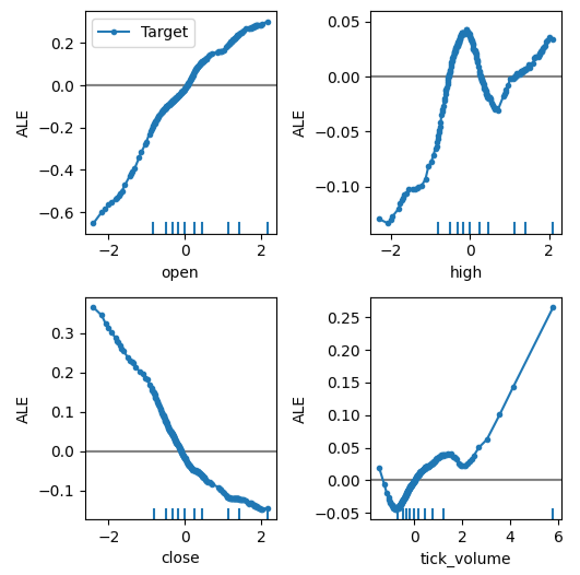

Fig 12: Visualizing our ALE Plots on our MetaTrader 5 Market Data

We shall now perform forward-selection. The algorithm starts with a null model and iteratively adds 1 feature that will improve the model's performance the most, until the model's performance cannot be increased further.

#Forward selection
from mlxtend.feature_selection import SequentialFeatureSelector as SFS
from mlxtend.plotting import plot_sequential_feature_selection as plot_sfs

Initialize the model.

#Reinitialize the model
all_nn  = MLPRegressor(hidden_layer_sizes=(10,20,40),max_iter=500)

Now we need to specify the forward-selection object we want. We shall instruct this instance of the algorithm to select as many variables as it finds important.

#Define the feature selector
sfs1 = SFS(all_nn,
           k_features=(1,X.shape[1]),
           forward=True,
           scoring='neg_mean_squared_error',
           cv=5,
           n_jobs=-1
          )

None of the FRED time-series were selected by the algorithm.

#Best features we identified
sfs1.k_feature_names_

('open', 'high', 'low')

We can visualize the algorithm's selection process. Our plot clearly shows that our model's performance diminished as we increased the model parameters.

#Fit the forward selection algorithm
fig1 = plot_sfs(sfs1.get_metric_dict(), kind='std_dev')

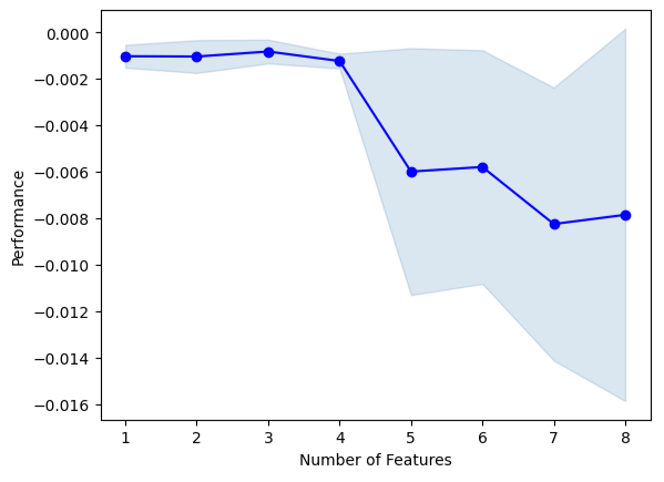
Fig 13: Visualizing our model's performance as we iteratively add more predictors

Parameter Tuning

Let us perform parameter tuning on our DNN model using a random search. First, we need to initialize our model.

#Reinitialize the model
model  = MLPRegressor(max_iter=500)

Now we shall define our tuning parameters.

#Define the tuner
tuner = RandomizedSearchCV(
        model,
        {
        "activation" : ["relu","logistic","tanh","identity"],
        "solver":["adam","sgd","lbfgs"],
        "alpha":[0.1,0.01,0.001,0.0001,0.00001,0.00001,0.0000001],
        "tol":[0.1,0.01,0.001,0.0001,0.00001,0.000001,0.0000001],
        "learning_rate":['constant','adaptive','invscaling'],
        "learning_rate_init":[0.1,0.01,0.001,0.0001,0.00001,0.000001,0.0000001],
        "hidden_layer_sizes":[(10,20,40),(10,20,40,80),(5,10,20,100),(100,50,10),(20,20,10),(1,5,10,20),(20,10,5,1)],
        "early_stopping":[True,False],
        "warm_start":[True,False],
        "shuffle": [True,False]
        },
        n_iter=500,
        cv=5,
        n_jobs=-1,
        scoring="neg_mean_squared_error"
)

Fit the tuning object.

#Fit the tuner
tuner.fit(train_X,train_y)

Let's see the best parameters we have found.

#The best parameters we found
tuner.best_params_

{'warm_start': False,
'tol': 1e-05,
'solver': 'lbfgs',
'shuffle': True,
'learning_rate_init': 0.01,
'learning_rate': 'invscaling',
'hidden_layer_sizes': (10, 20, 40, 80),
'early_stopping': True,
'alpha': 0.1,
'activation': 'relu'}

Deeper Parameter Optimization

Let us search for better model parameters using the SciPy library. We can imagine optimization processes as search problems, almost like the childhood game of hide and seek. You see, the ideal parameters for our model that will produce the best error rate on data the model has not seen before are hidden, in the infinite space of possible values we could assign to each of our continuous parameters.

Let us import the libraries we need.

#Deeper optimization
from scipy.optimize import minimize
from sklearn.metrics import mean_squared_error
from sklearn.model_selection import TimeSeriesSplit

Define a time-series split object.

#Define the time series split object
tscv = TimeSeriesSplit(n_splits=5,gap=look_ahead)

Create a data-frame to return the current cost, and create a list to store our model's progress for visualization.

#Create a dataframe to store our accuracy
current_error_rate = pd.DataFrame(index = np.arange(0,5),columns=["Current Error"])
algorithm_progress = []

Now we shall define our cost function. SciPy's minimize library offers us various algorithms to find the inputs to any function, that will result in the minimum output from the function. We will use average of the model's 5-fold error level on training data as the quantity to be minimized, while holding all other DNN parameters constant.

#Define the objective function
def objective(x):
    #The parameter x represents a new value for our neural network's settings
    model = MLPRegressor(hidden_layer_sizes=tuner.best_params_["hidden_layer_sizes"],
                         early_stopping=tuner.best_params_["early_stopping"],
                         warm_start=tuner.best_params_["warm_start"],
                         max_iter=500,
                         activation=tuner.best_params_["activation"],
                         learning_rate=tuner.best_params_["learning_rate"],
                         solver=tuner.best_params_["solver"],
                         shuffle=tuner.best_params_["shuffle"],
                         alpha=x[0],
                         tol=x[1],
                         learning_rate_init=x[2]
                         )
    #Now we will cross validate the model
    for i,(train,test) in enumerate(tscv.split(train_X)):
        #Train the model
        model.fit(train_X.loc[train[0]:train[-1],:],train_y.loc[train[0]:train[-1]])
        #Measure the RMSE
        current_error_rate.iloc[i,0] = mean_squared_error(train_y.loc[test[0]:test[-1]],model.predict(train_X.loc[test[0]:test[-1],:]))
    #Store the algorithm's progress
    algorithm_progress.append(current_error_rate.iloc[:,0].mean())
    #Return the Mean CV RMSE
    return(current_error_rate.iloc[:,0].mean())

Let us define starting points for the routine, and also specify any bounds for the parameters. For this problem, our only bounds are that all model parameters should be positive.

#Define the starting point
pt = [tuner.best_params_["alpha"],tuner.best_params_["tol"],tuner.best_params_["learning_rate_init"]]
bnds = ((10.00 ** -100,10.00 ** 100),
        (10.00 ** -100,10.00 ** 100),
        (10.00 ** -100,10.00 ** 100))

We will use the Truncated Newton Constrained (TNC) algorithm to optimize our model parameters. Truncated Newton methods are a family of methods suitable for solving large non-linear optimization problems subject to bounds. The SciPy library provides us with a wrapper to a C implementation of the algorithm.

#Searching deeper for parameters
result = minimize(objective,pt,method="TNC",bounds=bnds)

Let us see if we completed the terminated successfully.

#The result of our optimization
result

message: Linear search failed
success: False
status: 4
     fun: 0.001911232280110637
       x: [ 1.000e-100 1.000e-100 1.000e-100]
     nit: 0
     jac: [ 2.689e+06 9.227e+04 1.124e+05]
    nfev: 116

It appears we had difficulty finding optimal inputs, let us visualize the performance of our optimization procedure.

#Store the optimal coefficients
optimal_weights = result.x
optima_y = min(algorithm_progress)
optima_x = algorithm_progress.index(optima_y)
inputs = np.arange(0,len(algorithm_progress))

#Plot the performance of our optimization procedure
plt.scatter(inputs,algorithm_progress)
plt.plot(optima_x,optima_y,'ro',color='r')
plt.axvline(x=optima_x,ls='--',color='red')
plt.axhline(y=optima_y,ls='--',color='red')
plt.xlabel("Iterations")
plt.ylabel("Training MSE")
plt.title("Minimizing Training Error")

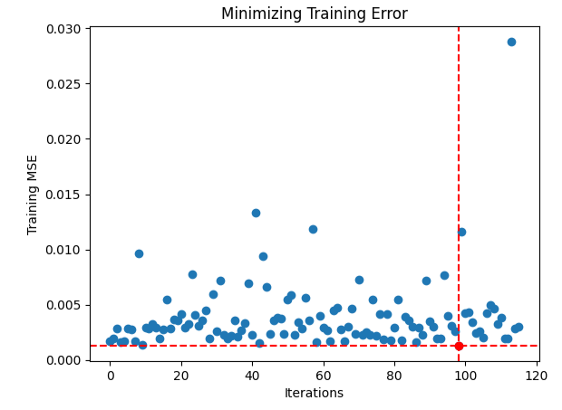
Fig 14: The red dot represents the optimal input values estimated by our TNC optimizer

Testing For Overfitting

Let us initialize all 3 of our models and see if we can train them on the training set and outperform the default model on test data. Recall that we have not used the test data in our decision-making process thus far.

#Testing for overfitting
default_nn = MLPRegressor(max_iter=500)

#Randomized NN
random_search_nn = MLPRegressor(hidden_layer_sizes=tuner.best_params_["hidden_layer_sizes"],
                         early_stopping=tuner.best_params_["early_stopping"],
                         warm_start=tuner.best_params_["warm_start"],
                         max_iter=500,
                         activation=tuner.best_params_["activation"],
                         learning_rate=tuner.best_params_["learning_rate"],
                         solver=tuner.best_params_["solver"],
                         shuffle=tuner.best_params_["shuffle"],
                         alpha=tuner.best_params_["alpha"],
                         tol=tuner.best_params_["tol"],
                         learning_rate_init=tuner.best_params_["learning_rate_init"]
                         )

#TNC NN
tnc_nn = MLPRegressor(hidden_layer_sizes=tuner.best_params_["hidden_layer_sizes"],
                         early_stopping=tuner.best_params_["early_stopping"],
                         warm_start=tuner.best_params_["warm_start"],
                         max_iter=500,
                         activation=tuner.best_params_["activation"],
                         learning_rate=tuner.best_params_["learning_rate"],
                         solver=tuner.best_params_["solver"],
                         shuffle=tuner.best_params_["shuffle"],
                         alpha=result.x[0],
                         tol=result.x[1],
                         learning_rate_init=result.x[2]
                         )

Fit each of the models on the training set.

#Store the models in a list
models = [default_nn,random_search_nn,tnc_nn]

#Fit the models
for model in models:
    model.fit(train_X,train_y)

Create a data-frame to store our validation error levels.

#Create a dataframe to store our validation error
validation_error = pd.DataFrame(columns=["Default","Randomized","TNC"],index=np.arange(0,5))

Test each model and record its score.

#Let's obtain our cv score
default_score = cross_val_score(default_nn,test_X,test_y,scoring='neg_root_mean_squared_error',cv=5,n_jobs=-1)
random_score = cross_val_score(random_search_nn,test_X,test_y,scoring='neg_root_mean_squared_error',cv=5,n_jobs=-1)
tnc_score = cross_val_score(tnc_nn,test_X,test_y,scoring='neg_root_mean_squared_error',cv=5,n_jobs=-1)

#Store the model error in a dataframe
for i in np.arange(0,5):
    validation_error.iloc[i,0] = default_score[i]
    validation_error.iloc[i,1] = random_score[i]
    validation_error.iloc[i,2] = tnc_score[i]

Let's see the validation error.

#Let's see the validation error
validation_error

Default Model	Random Search	TNC
-0.362851	-0.029476	-0.054709
-0.323601	-0.053967	-0.087707
-0.064432	-0.024282	-0.026481
-0.121226	-0.019693	-0.017709
-0.064801	-0.012812	-0.016125

Calculating our average performance across all 5-folds clearly shows that our random search model is our best bet.

#Our best performing model
validation_error.mean()

Model	Average Validation Error
Default Model	-0.187382
Random Search	-0.028046
TNC	-0.040546

Creating box-plots quickly shows us the extent to which the default model's performance varied. Our customized models managed to perform within a tight band of error levels, giving us more confidence in our parameter tuning choices.

#Let's create box-plots
sns.boxplot(validation_error)

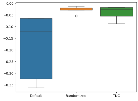
Fig 15: Visualizing our model's performance as box-plots

Creating line plots of the cross-validation data highlights the disparity between the default model and our tuned models. We can see there is a significant amount of error between the blue line representing the default model's performance and the remaining colored plots.

#We can also visualize model performance through a line plot
validation_error.plot()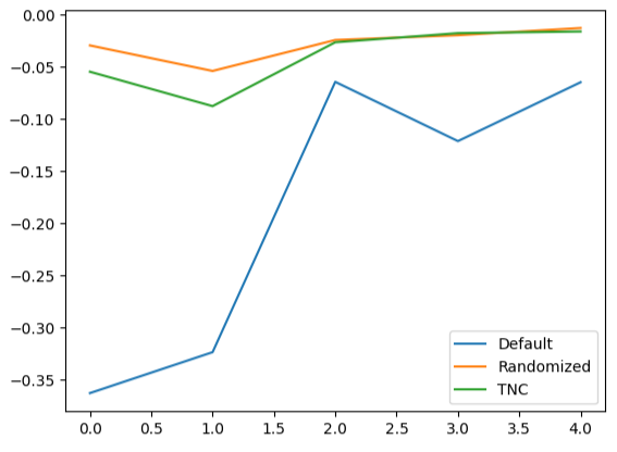

Fig 16: Plotting our different models 5-fold performance on test data

Residuals Analysis

We cannot blindly trust our model and deploy it into production. Let us try to ensure that our model has actually learned effectively by inspecting the residuals of our model. Ideally, a model that has perfectly approximated a function will have residuals that are a flat line. Meaning there is no error in the model's prediction. Additionally, this also implies that the amount of error in the model's prediction does not change.

Consequently, the further away our model's performance is from the ideal, the more distortion we will observe from the ideal linear and stationary residual plot. Our model's residuals displayed varying amount of error, that at times was correlated with the previous amount of error. This is probable cause for concern and may be potentially addressed by transforming the predictor or the target.

Let us initialize the model.

#Resdiuals analysis
model = MLPRegressor(hidden_layer_sizes=tuner.best_params_["hidden_layer_sizes"],
                         early_stopping=tuner.best_params_["early_stopping"],
                         warm_start=tuner.best_params_["warm_start"],
                         max_iter=500,
                         activation=tuner.best_params_["activation"],
                         learning_rate=tuner.best_params_["learning_rate"],
                         solver=tuner.best_params_["solver"],
                         shuffle=tuner.best_params_["shuffle"],
                         alpha=tuner.best_params_["alpha"],
                         tol=tuner.best_params_["tol"],
                         learning_rate_init=tuner.best_params_["learning_rate_init"]
                         )

Fit the model on the training data, and then record the residuals using the test data.

#Fit the model
model.fit(train_X,train_y)

#Record the residuals
residuals = test_y - model.predict(test_X)

Our residuals plot were far from the ideal, and we may need to explore other preprocessing steps to address this.

#Residuals analysis
residuals.plot()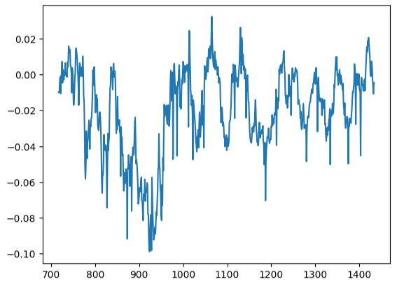

Fig 17: Visualizing our model's residuals on test data

Measuring auto-correlation is a robust approach to detecting possible spurious regressions. Unfortunately, our model residuals failed this test too and could possibly serve as an indicator that we can gain additional enhancements if we better transformed our predictors or target.

#Autocorrelation plot
from statsmodels.graphics.tsaplots import plot_acf
acf = plot_acf(residuals,lags=40)

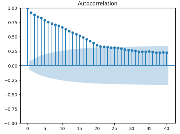
Fig 18: Visualizing our model's residuals

Preparing To Export To ONNX

Before we can export our data to ONNX format, let us first store the mean values and standard deviations of each column into a data-frame. Note, since we did not gain any improvements from transforming the data into percent changes, we will instead use the data in its original form and use that for our z-score calculations.

#Prepare to convert the model to ONNX format
scale_factors = pd.DataFrame(columns=X.columns,index=["mean","std"])
for i in X.columns:
    scale_factors.loc["mean",i] = merged_data.loc[:,i].mean()
    scale_factors.loc["std",i]  = merged_data.loc[:,i].std()
    merged_data.loc[:,i] = (merged_data.loc[:,i] - scale_factors.loc["mean",i]) / scale_factors.loc["std",i]

scale_factors

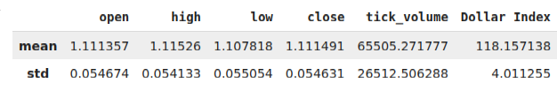
Fig 19: Our data-frame with our z-scores

Write out the data to CSV format.

#Save the scale factors to CSV format
scale_factors.to_csv("FRED EURUSD D1 scale factors.csv")

Exporting To ONNX

ONNX is an open-source protocol that allows developers to build and deploy machine learning models in any programming language that supports the ONNX API. We shall first import the libraries we need.

# Import the libraries we need
import onnx
from skl2onnx import convert_sklearn
from skl2onnx.common.data_types import FloatTensorType

Initialize the model, for the last time.

#Initialize the model
model = MLPRegressor(hidden_layer_sizes=tuner.best_params_["hidden_layer_sizes"],
                         early_stopping=tuner.best_params_["early_stopping"],
                         warm_start=tuner.best_params_["warm_start"],
                         max_iter=500,
                         activation=tuner.best_params_["activation"],
                         learning_rate=tuner.best_params_["learning_rate"],
                         solver=tuner.best_params_["solver"],
                         shuffle=tuner.best_params_["shuffle"],
                         alpha=tuner.best_params_["alpha"],
                         tol=tuner.best_params_["tol"],
                         learning_rate_init=tuner.best_params_["learning_rate_init"]
                         )

Fit the model on all the data we have.

# Fit the model on all the data we have
model.fit(merged_data.loc[:,predictors],merged_data.loc[:,target])

Define the output shape of our model.

# Define the input type
initial_types = [("float_input",FloatTensorType([1,X.shape[1]]))]

Create an ONNX graph representation of our model.

# Create the ONNX representation
onnx_model = convert_sklearn(model,initial_types=initial_types,target_opset=12)

Save the ONNX model.

# Save the ONNX model
onnx.save_model(onnx_model,"FRED EURUSD D1.onnx")

Visualizing Our Model in Netron

Visualizing our model will help us validate that it has been created according to our specifications. We want to validate that the input and output shapes are in line with our expectations. Netron is an open-source library for visualizing machine learning models. Let us import the library to get started.

import netron

Now we can easily visualize our DNN Regressor.

netron.start("FRED EURUSD D1.onnx")

Visualizing our ONNX model

Fig 20: Visualizing our DNN Regressor

Our model specifications

Fig 21: Visualizing our model's input and output shapes

Implementation in MQL5

The first component we need to integrate into our Expert Advisor will be the ONNX model. We will simply include the ONNX file as a resource for our Expert Advisor.

//+------------------------------------------------------------------+
//|                                               FRED EURUSD AI.mq5 |
//|                                        Gamuchirai Zororo Ndawana |
//|                          https://www.mql5.com/en/gamuchiraindawa |
//+------------------------------------------------------------------+
#property copyright "Gamuchirai Zororo Ndawana"
#property link      "https://www.mql5.com/en/gamuchiraindawa"
#property version   "1.00"

//+------------------------------------------------------------------+
//| Require the ONNX file                                            |
//+------------------------------------------------------------------+
#resource "\\Files\\FRED EURUSD D1.onnx" as const uchar onnx_buffer[];

Now let us load the trade library that we need for managing our positions.

//+------------------------------------------------------------------+
//| Libraries                                                        |
//+------------------------------------------------------------------+
#include  <Trade/Trade.mqh>
CTrade Trade;

Creating global variables we will need throughout our program.

//+------------------------------------------------------------------+
//| Define global variables                                          |
//+------------------------------------------------------------------+
long    model;
double  mean_values[5] = {1.1113568153310105,1.1152603484320558,1.1078179790940768,1.1114909337979093,65505.27177700349};
double  std_values[5]  = {0.05467420688685988,0.05413287747761819,0.05505429755411189,0.054630920048519924,26512.506288360997};
vectorf model_output   = vectorf::Zeros(1);
vectorf model_inputs   = vectorf::Zeros(8);
int     model_sate     = 0;
int     system_sate    = 0;
double  bid,ask;

Whenever our model has been loaded for the first time, let us first try to load our ONNX model and then test if it's working.

//+------------------------------------------------------------------+
//| Expert initialization function                                   |
//+------------------------------------------------------------------+
int OnInit()
  {
//--- Load the ONNX model
   if(!load_onnx_model())
     {
      //--- We failed to load the ONNX model
      return(INIT_FAILED);
     }

//--- Test if we can get a prediction from our model
   model_predict();

//--- Eveything went fine
   return(INIT_SUCCEEDED);
  }

If our model is removed from the chart, we will also free up the resources we are no longer using.

//+------------------------------------------------------------------+
//| Expert deinitialization function                                 |
//+------------------------------------------------------------------+
void OnDeinit(const int reason)
  {
//--- Release the resources we no longer need
   release_resources();
  }

Whenever we receive new prices, we will update the variables we have assigned to store current market prices. Likewise, if we have no open positions, we will follow our model's directive. On the other hand, if we already have open positions, then we will allow our model to warn us about possible reversals, and we will close our positions accordingly.

//+------------------------------------------------------------------+
//| Expert tick function                                             |
//+------------------------------------------------------------------+
void OnTick()
  {
//--- Update our bid and ask prices
   update_market_prices();

//--- Fetch an updated prediction from our model
   model_predict();

//--- If we have no trades, follow our model's directions.
   if(PositionsTotal() == 0)
     {
      //--- Our model is predicting price levels will appreciate
      if(model_sate == 1)
        {
         Trade.Buy(0.3,"EURUSD",ask,0,0,"FRED EURUSD AI");
         system_sate = 1;
        }
      //--- Our model is predicting price levels will deppreciate
      if(model_sate == -1)
        {
         Trade.Sell(0.3,"EURUSD",ask,0,0,"FRED EURUSD AI");
         system_sate = -1;
        }
     }

//--- Otherwise Manage our open positions
   else
     {
      if(system_sate != model_sate)
        {
         Alert("AI System Detected A Reversal! Closing All Positions on EURUSD");
         Trade.PositionClose("EURUSD");
        }
     }

  }
//+------------------------------------------------------------------+

This function will update our variables that keep track of the current market prices.

//+------------------------------------------------------------------+
//| Update market prices                                             |
//+------------------------------------------------------------------+
void update_market_prices(void)
  {
   bid = SymbolInfoDouble(Symbol(),SYMBOL_BID);
   ask = SymbolInfoDouble(Symbol(),SYMBOL_ASK);
  }

Now we will define the fashion in which our resources should be released.

//+------------------------------------------------------------------+
//| Release the resources we no longer need                          |
//+------------------------------------------------------------------+
void release_resources(void)
  {
   OnnxRelease(model);
   ExpertRemove();
  }

Let us define the function responsible for creating our ONNX model from the buffer we created above. If this function fails at any point, it will return false which will break our initialization procedure.

//+------------------------------------------------------------------+
//| Create our ONNX model from the buffer we defined above           |
//+------------------------------------------------------------------+
bool load_onnx_model(void)
  {
//--- Create the ONNX model from the buffer we defined
   model = OnnxCreateFromBuffer(onnx_buffer,ONNX_DEFAULT);

//--- Validate the model was not illdefined
   if(model == INVALID_HANDLE)
     {
      //--- We failed to define our model
      Comment("We failed to create our ONNX model: ",GetLastError());
      return false;
     }

//---- Define the model I/O shape
   ulong input_shape[] = {1,8};
   ulong output_shape[] = {1,1};
//--- Validate our model's I/O shapes
   if(!OnnxSetInputShape(model,0,input_shape) || !OnnxSetOutputShape(model,0,output_shape))
     {
      Comment("Failed to define our model I/O shape: ",GetLastError());
      return(false);
     }
//--- Everything went fine!
   return(true);
  }

This is the function responsible for fetching a prediction from our model. The function will first fetch and normalize EURUSD market data quotes, before calling a routine responsible for reading our current FRED alternative data.

//+------------------------------------------------------------------+
//| This function will fetch a prediction from our model             |
//+------------------------------------------------------------------+
void model_predict(void)
  {
//--- Get the input data ready
   for(int i =0; i < 6; i++)
     {
      //--- The first 5 inputs will be fetched from the market
      matrix eur_usd_ohlc = matrix::Zeros(1,5);
      eur_usd_ohlc[0,0] = iOpen(Symbol(),PERIOD_D1,0);
      eur_usd_ohlc[0,1] = iHigh(Symbol(),PERIOD_D1,0);
      eur_usd_ohlc[0,2] = iLow(Symbol(),PERIOD_D1,0);
      eur_usd_ohlc[0,3] = iClose(Symbol(),PERIOD_D1,0);
      eur_usd_ohlc[0,4] = iTickVolume(Symbol(),PERIOD_D1,0);
      //--- Fill in the data
      if(i<4)
        {
         model_inputs[i] = (float)((eur_usd_ohlc[0,i] - mean_values[i])/ std_values[i]);
        }
      //--- We have to read in the fred alternative data
      else
        {
         read_fred_data();
        }
     }
  }
//+------------------------------------------------------------------+

This function will read our FRED alternative data from our MQL5\Files directory. Recall that the CSV file will be updated every day by our Python script.

//+------------------------------------------------------------------+
//| This function will read in our FRED data                         |
//+------------------------------------------------------------------+
bool read_fred_data(void)
  {
//--- Read in the file
   string file_name = "FRED EURUSD ALT DATA.csv";

//--- Try open the file
   int result = FileOpen(file_name,FILE_READ|FILE_CSV|FILE_ANSI,","); //Strings of ANSI type (one byte symbols).

//--- Check the result
   if(result != INVALID_HANDLE)
     {
      Print("Opened the file");
      //--- Store the values of the file

      int counter = 0;
      string value = "";
      while(!FileIsEnding(result) && !IsStopped()) //read the entire csv file to the end
        {
         if(counter > 20)   //if you aim to read 10 values set a break point after 10 elements have been read
            break;          //stop the reading progress

         value = FileReadString(result);
         Print("Counter: ");
         Print(counter);
         Print("Trying to read string: ",value);

         if(counter == 3)
           {
            model_inputs[5] = (float) value;
           }

         if(counter == 5)
           {
            model_inputs[6] = (float) value;
           }

         if(counter == 7)
           {
            model_inputs[7] = (float) value;
           }

         if(FileIsLineEnding(result))
           {
            Print("row++");
           }

         counter++;
        }

      //--- Show the input and Fred data
      Print("Input Data: ");
      Print(model_inputs);
      //---Close the file
      FileClose(result);
      //--- Store the model prediction
      OnnxRun(model,ONNX_DEFAULT,model_inputs,model_output);
      Comment("Model Forecast: ",model_output[0]);
      if(model_output[0] > iClose(Symbol(),PERIOD_D1,0))
        {
         model_sate = 1;
        }

      else
        {
         model_sate = -1;
        }

      //--- Everything went fine
      return(true);
     }

//--- We failed to find the file
   else
     {
      //--- Give the user feedback
      Print("We failed to find the file with the FRED data");
      return false;
     }

//--- Something went wrong
   return false;
  }

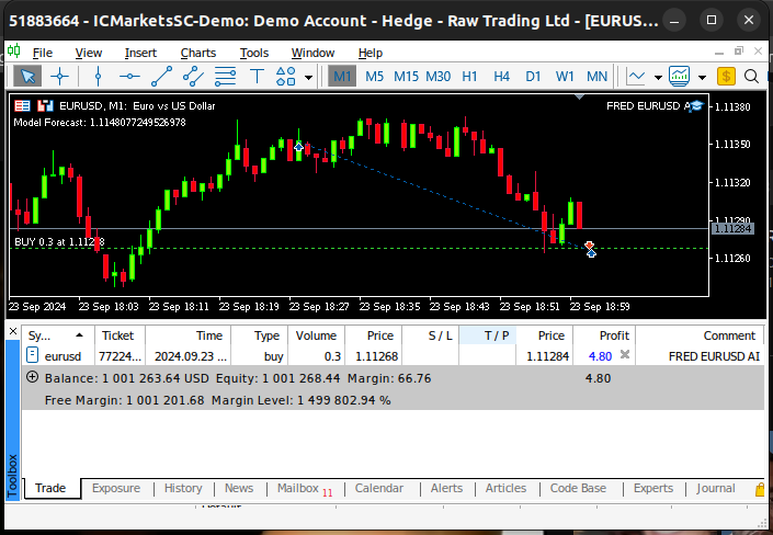
Fig 22: Forward testing our algorithm

Conclusion

In this article, we have demonstrated that the Nominal Broad Daily Index may either not be of much help when trying to forecast the EURUSD pair, or alternatively, the symbol may require more transformations before the true relationship can be learned effectively. Alternatively, we may also consider testing a wider variety of models to maximize our likelihood of capturing the relationship well. Models such as Support Vector Machines tend to perform well in problems that require learning a decision boundary in high dimensional space. There are hundreds of thousands of data sets we are still yet to explore. But unfortunately, we did not gain an edge over the rest of the market today.

Attached files |

Download ZIP

FRED_EURUSD_AI.mq5 (8.61 KB)

FRED_EURUSD_D1.onnx (18.9 KB)

Alternative_Data_EURUSD.ipynb (2502.45 KB)

Fetch_Fred_Data.ipynb (3.75 KB)

Visualizing_The_Deep_Neural_Network.ipynb (1.31 KB)

Warning: All rights to these materials are reserved by MetaQuotes Ltd. Copying or reprinting of these materials in whole or in part is prohibited.