Example of Stochastic Optimization and Optimal Control

Introduction to Stochastic Modeling and Control Optimization

Stochastic modeling and control optimization are mathematical methods that help solve problems under uncertainty. They are used in finance, engineering, artificial intelligence, and many other areas.

Stochastic modeling is used to describe systems with random elements, such as stock market price movements or a queue at a restaurant. It is based on random variables, probability distributions, and stochastic processes. Methods such as Monte Carlo and Markov chains can model these processes and predict their behavior.

Control optimization helps you find better solutions for controlling systems. It is used to automate and improve the operation of various processes, from driving cars to operating chemical plants. Basic methods include linear quadratic controller, model predictive control, and reinforcement learning. Stochastic control optimization combines both approaches and is applied to problems where decisions must be made in the absence of complete information about the future, for example, in investments or supply chain management.

These methods allow us to model uncertain systems and make informed decisions in complex environments, making them important tools in the modern world.

EA

The SMOC (Smart Money Optimal Control) advisor uses a combination of technical indicators, mathematical models and risk management methods to make trading decisions in the Forex market as a simple example demonstrating its capabilities.

Main characteristics:

1. Predictive Management Model: The EA uses an optimal management algorithm to predict future price movements and make trading decisions.
2. Adaptive parameters: the system adjusts the forecast horizon and lot size depending on market volatility and account drawdown.
3. Multiple technical indicators: Includes simple moving averages (SMA), parabolic SAR, relative strength index (RSI) and average true range (ATR) for trend and volatility analysis.
4. Dynamic Stop Loss and Take Profit: The EA calculates and updates SL and TP levels based on market volatility.
5. Risk Management: Includes functions for adjusting position size based on account balance and drawdown.

Possible areas of application:

• Medium and long term trading strategies
• Markets with pronounced trends
• Portfolios requiring complex risk management

Pros:

1. Adaptive approach: the system adapts to changing market conditions, potentially increasing its resilience.
2. Complex analysis: by combining multiple indicators and mathematical models, it aims to reflect various aspects of market behavior.
3. Risk accounting: the advisor includes protection against drawdowns and dynamic determination of position size.
4. Verbose logging: A log file is maintained for performance analysis and debugging.

Cons:

1. Complexity: Complex algorithms can make the system difficult to understand and optimize.
2. Computationally intensive: Optimal control calculations can be computationally intensive, potentially limiting their use on less powerful systems.
3. Potential overfitting: With a large number of parameters and indicators, there is a risk of overfitting to historical data.
4. Market Assumption: The strategy's effectiveness is based on the assumption that past price behavior can predict future movements, which is not always true in financial markets.

Main characteristics of the SMOC advisor

Model Predictive Control (MPC): The EA uses an optimal control algorithm to predict future price movements and make trading decisions. This is implemented in the OptimalControl() function.

//+------------------------------------------------------------------+
//| Function for optimal control using Model Predictive Control      |
//+------------------------------------------------------------------+
int OptimalControl( double currentPrice)
  {
   int predictionHorizon = CalculateAdaptiveHorizon();
   double mu = EstimateDrift();
   double sigma = EstimateVolatility();
   double baseThreshold = 0.001 ;
   double decisionThreshold = baseThreshold * ( 1 + ( 1 - successRate));
   double dt = 1.0 / 1440.0 ;

   double bestExpectedReturn = - DBL_MAX ;
   int bestDecision = 0 ;
   double bestU1 = 0 , bestU2 = 0 ;

// Optimize the search space
   double u1Start = 0.01 , u1End = 0.99 , u1Step = 0.01 ;
   double u2Start = 0.01 , u2End = 0.99 , u2Step = 0.01 ;

// Calculate historical average price
   int lookbackPeriod = 20 ; // You can adjust this
   double historicalPrices[];
   ArraySetAsSeries (historicalPrices, true );
   CopyClose ( Symbol (), PERIOD_CURRENT , 0 , lookbackPeriod, historicalPrices);
   double avgHistoricalPrice = ArraySum(historicalPrices) / lookbackPeriod;

   for ( double u1 = u1Start; u1 <= u1End; u1 += u1Step)
     {
       for ( double u2 = u2Start; u2 <= u2End; u2 += u2Step)
        {
         double expectedReturn = CalculateExpectedReturn(currentPrice, mu, sigma, dt, predictionHorizon, u1, u2);

         // Compare with historical average
         if (currentPrice > avgHistoricalPrice)
           {
            expectedReturn *= - 1 ; // Invert expected return to favor selling when price is high
           }

         if (expectedReturn > bestExpectedReturn)
           {
            bestExpectedReturn = expectedReturn;
            bestU1 = u1;
            bestU2 = u2;
           }
        }
     }

   LogMessage( StringFormat ( "OptimalControl - Best u1: %f, Best u2: %f, Best Expected Return: %f, Decision Threshold %f" ,
                           bestU1, bestU2, bestExpectedReturn, decisionThreshold));

   if (bestExpectedReturn > decisionThreshold)
       return 1 ; // Buy
   if (bestExpectedReturn < decisionThreshold)
       return - 1 ; // Sell
   return 0 ; // Hold
  }

This uses Model Predictive Control (MPC) to make optimal trading decisions. The OptimalControl function is the core of this algorithm, designed to determine whether to buy, sell or hold based on current market conditions and forecasts.

The OptimalControl function takes the current price as input and returns an integer representing the trading decision:

• 1 for purchase
• -1 for sale
• 0 to hold

Key Components

1. Adaptive Forecast Horizon: The function calculates an adaptive forecast horizon, allowing the algorithm to adjust the forecast range depending on market conditions.
2. Market Parameter Assessment: Assesses key market parameters:
   • Drift (μ): Expected return of an asset
   • Volatility (σ): the rate of change in the price of an asset.
3. Decision Threshold: The dynamic threshold is calculated based on the base threshold and the success rate of the algorithm. This adapts the sensitivity of the algorithm to market changes.
4. Optimization process: The function uses grid search to optimize two control parameters (u1 and u2) in a defined search space.
5. Historical Price Comparison: The current price is compared to the historical average to adjust the strategy depending on whether the current price is relatively high or low.
6. Calculating expected return: For each combination of control parameters, the expected return is calculated using a separate function (not shown in this code snippet).
7. Decision making: Based on the best expected return and the decision threshold, a decision is made whether to buy, sell or hold the asset.

Detailed review

1. The function starts by initializing variables and calculating the required parameters.
2. It then enters a nested loop to find the optimal control parameters (u1 and u2).
3. For each combination of u1 and u2, the expected return is calculated.
4. If the current price is above the historical average, it inverts the expected return. This creates a bias towards selling when prices are high and buying when prices are low.
5. It tracks the best expected return and the corresponding benchmarks.
6. After optimization, the best parameters and expected profitability are recorded.
7. Finally, it compares the best expected return with the threshold value for making a trading decision.

Key ideas

• The algorithm adapts to market conditions using an adaptive horizon and a dynamic threshold.
• It involves both short-term optimization (using the MPC approach) and long-term understanding of trends (using historical price comparisons).
• Using grid search for optimization allows for a thorough exploration of the parameter space, potentially leading to more robust decisions.

Possible improvements

1. Grid search can be replaced with a more efficient optimization algorithm to improve performance.
2. Comparison of historical prices can be made more complex, perhaps by including multiple time frames.
3. Risk management features can be added to balance return optimization with risk minimization.

 /+------------------------------------------------------------------+
//| Calculate expected return for given parameters                   |
//+------------------------------------------------------------------+
double CalculateExpectedReturn( double currentPrice, double mu, double sigma, double dt, int horizon, double u1, double u2)
  {
   double tempPrice = currentPrice;
   double totalReturn = 0 ;

   for ( int i = 0 ; i < horizon; i++)
     {
       double Z = MathSqrt (- 2.0 * MathLog (u1)) * MathCos ( 2.0 * M_PI * u2);
       double nextPrice = tempPrice * MathExp ((mu - 0.5 * sigma * sigma) * dt + sigma * MathSqrt (dt) * Z);
      totalReturn += nextPrice - tempPrice;
      tempPrice = nextPrice;
     }

   return totalReturn / horizon;
  }

It is a critical component in financial models and algorithmic trading systems. This function estimates the expected return of an asset over a specified time horizon using a stochastic process known as geometric Brownian motion (GBM).

 double CalculateExpectedReturn( double currentPrice, double mu, double sigma, double dt, int horizon, double u1, double u2)

Parameters

1. currentPrice : Current price of the asset
2. mu : Drift parameter (expected return)
3. sigma: volatility parameter
4. dt: Time step (usually 1/number of steps per year)
5. Horizon: The number of time steps to simulate.
6. u1, u2: Random numbers used to generate normally distributed random variables.

Overview of functions

This function models the price path of an asset using the geometric Brownian motion model, which is widely used in financial mathematics to model stock prices. It then calculates the average return along the modeled path.

Detailed explanation

1. Initialization:
   • tempPrice is initialized to the current price.
   • totalReturn is set to 0 to accumulate returns.
2. Simulation loop: The function enters a loop that traverses the horizon times. In each iteration: a. Generate a random normal variable :

 double Z = MathSqrt (- 2.0 * MathLog (u1)) * MathCos ( 2.0 * M_PI * u2);

This line implements the Box-Muller transform to generate a standard normal random variable. This is a key component in modeling a random walk in asset prices.

Calculate the next price:

 double nextPrice = tempPrice * MathExp ((mu - 0.5 * sigma * sigma) * dt + sigma * MathSqrt (dt) * Z);

This line implements the formula for geometric Brownian motion:

• (mu - 0.5 * sigma * sigma) * dt is the drift component
• sigma * MathSqrt(dt) * Z is the random shock component

Cumulative return:

totalReturn += nextPrice - tempPrice;

The function calculates and accumulates the return for each step.

Price update:

tempPrice = nextPrice;

The current price is updated for the next iteration.

Calculate the average yield:

 return totalReturn / horizon;

The function returns the average return over the simulated horizon.

Importance in financial modeling

1. Risk Assessment: By simulating multiple price paths, this feature helps assess the potential risks associated with an asset.
2. Option Pricing: This type of modeling is fundamental in option pricing models, especially Monte Carlo methods.
3. Portfolio optimization: Expected returns are key inputs in portfolio optimization algorithms.
4. Trading Strategies: Algorithmic trading strategies often use expected returns to make buy/sell decisions.

Limitations and Considerations

1. Model Assumptions: The GBM model assumes that returns are normally distributed and independent, which may not always be true in real markets.
2. Parameter estimation: The accuracy of the function depends largely on the correct estimation of mu and sigma.
3. Single Simulation: This function performs a single simulation. In practice, multiple simulations are often run to obtain a more reliable estimate.
4. Time horizon: The choice of horizon and dt can significantly affect the results and should be chosen carefully based on the specific use case.

This function is a fundamental building block in quantitative finance, providing a way to estimate future returns based on current market parameters. Its implementation in trading algorithms enables data-driven decision making in complex financial environments.

Adaptive parameters: the system adjusts its forecast horizon and lot size based on market volatility and account drawdown. This is achieved using functions such as CalculateAdaptiveHorizon() and AdjustLotSizeForDrawdown().

//+------------------------------------------------------------------+
//| Calculate adaptive horizon                                       |
//+------------------------------------------------------------------+
int CalculateAdaptiveHorizon()
  {
   double currentVolatility = EstimateVolatility();
   int baseHorizon = 5 ;
   return MathMax (baseHorizon, MathMin ( 20 , ( int )(baseHorizon * ( 1 + currentVolatility))));
  }

 // Función para ajustar el tamaño del lote basado en drawdown
double AdjustLotSizeForDrawdown()
  {
   static int consecutiveLosses = 0 ;
   static double maxBalance = 0 ;

   double currentBalance = AccountInfoDouble ( ACCOUNT_BALANCE );
   double currentEquity = AccountInfoDouble ( ACCOUNT_EQUITY );

   if (currentBalance > maxBalance)
      maxBalance = currentBalance;

   double drawdown = (maxBalance - currentEquity) / maxBalance;

   double baseLotSize = CalculateDynamicLotSize();

   if (drawdown > 0.1 ) // 10% drawdown
     {
       return baseLotSize * 0.5 ; // Reducir el tamaño del lote a la mitad
     }
   else
       if (consecutiveLosses > 3 )
        {
         return baseLotSize * 0.75 ; // Reducir el tamaño del lote en un 25%
        }

   return baseLotSize;
  }

This is an important component of trading risk management. This feature adjusts the trading lot size based on the current account drawdown and the number of consecutive losses.

Overview of functions

The AdjustLotSizeForDrawdown function is designed to dynamically adjust the trading lot size to manage risks in volatile market conditions. It takes into account two main factors:

1. Current drawdown of the trading account
2. Number of consecutive defeats

Key Components

1. Static variables:
   • Therefore Losses: tracks the number of consecutive losing trades
   • maxBalance: maintains the maximum balance reached on the account
2. Account Information:
   • currentBalance: Current balance of the trading account
   • currentEquity: Current equity of the trading account
3. Drawdown calculation : Drawdown is calculated as a percentage decrease from the maximum balance to the current equity.
4. Base Lot Size: The function calls CalculateDynamicLotSize() (not shown in this snippet) to determine the base lot size.
5. Lot Size Adjustment: The function adjusts the lot size based on two conditions:
• If the drawdown exceeds 10%
• If there were more than 3 consecutive losses

Detailed explanation

Maximum balance update:

 if (currentBalance > maxBalance)
   maxBalance = currentBalance;

This allows you to track the maximum balance achieved, which is crucial for calculating drawdown.

Calculation of drawdown:

 double drawdown = (maxBalance - currentEquity) / maxBalance;

This calculates the current drawdown as a percentage of the maximum balance.

Getting the base lot size:

 double baseLotSize = CalculateDynamicLotSize();

This calls a separate function to calculate the initial lot size.

Adjustment for high drawdown:

 if (drawdown > 0.1 ) // 10% drawdown
  {
   return baseLotSize * 0.5 ; // Reduce lot size by half
  }

If the drawdown exceeds 10%, the function reduces the lot size by half to reduce the risk.

Consecutive Loss Adjustment:

 else if (consecutiveLosses > 3 )
  {
   return baseLotSize * 0.75 ; // Reduce lot size by 25%
  }

If there were more than 3 consecutive losses, the function reduces the lot size by 25%.

Return Default: If none of the conditions are met, the function returns the base lot size without adjustment.

Importance in risk management:

1. Drawdown Protection: By reducing lot sizes during significant drawdowns, this feature helps protect the account from further losses during adverse market conditions.
2. Managing Losing Streaks: Adjusting for consecutive losses helps mitigate the effects of losing streaks, which can be devastating psychologically and financially.
3. Dynamic Risk Adjustment: This feature allows you to dynamically manage your risks by adjusting to current market conditions and trading results.

Considerations and potential improvements

1. Gradual Adjustment: The feature can be modified to implement a more gradual adjustment of lot sizes based on different levels of drawdown.
2. Recovery Mechanism: An additional mechanism can be added to gradually increase lot sizes as the account recovers from a drawdown.
3. Maximum Lot Size: Introducing a maximum lot size limit can provide an additional layer of risk management.
4. Win Tracking: The feature can be expanded to track consecutive wins and potentially increase lot sizes during favorable periods.

This feature is a vital aspect of risk management in trading systems, helping to preserve capital in difficult market conditions and mitigate the effects of losing streaks.

Several technical indicators: the advisor includes several technical indicators for analysis:

• Simple Moving Averages (SMA)
• Parabolic SAR
• Relative Strength Index (RSI)
• Average True Range (ATR)

 // Initialize indicator handles
   smaHandle = iMA ( Symbol (), PERIOD_CURRENT , 50 , 0 , MODE_SMA , PRICE_CLOSE );
   psarHandle = iSAR ( Symbol (), PERIOD_CURRENT , 0.02 , 0.2 );
   rsiHandle = iRSI ( Symbol (), PERIOD_CURRENT , 14 , PRICE_CLOSE );
   atrHandle = iATR ( Symbol (), PERIOD_CURRENT , 14 );

Dynamic Stop Loss and Take Profit: The EA calculates and updates SL and TP levels based on market volatility using the CalculateDynamicSL() and CalculateDynamicTP() functions.

 double CalculateDynamicSL( double price, int decision)
  {
   double atrValue[];
   if ( CopyBuffer (atrHandle, 0 , 0 , 1 , atrValue) <= 0 )
     {
      LogMessage( StringFormat ( "Error getting ATR values: %d" , GetLastError ()));
       return 0.0 ;
     }
   double volatility = atrValue[ 0 ];
   double dynamicSL = (decision == 1 ) ? price - (volatility * multi * 1.2 ) : price + (volatility * multi * 0.8 );

   return NormalizeDouble (dynamicSL, _Digits );
  }


double CalculateDynamicTP( double price, int decision)
  {
   double atrValue[];
   if ( CopyBuffer (atrHandle, 0 , 0 , 1 , atrValue) <= 0 )
     {
      LogMessage( StringFormat ( "Error getting ATR values: %d" , GetLastError ()));
       return 0.0 ;
     }
   double volatility = atrValue[ 0 ];
   double dynamicTP = (decision == 1 ) ? price + (volatility * multi * 1.8 ) : price - (volatility * multi * 2.2 );

   return NormalizeDouble (dynamicTP, _Digits );
  }

This feature calculates dynamic stop loss (SL) and take profit (TP) levels based on current market volatility, improving risk management and potentially improving trading results.

Feature Reviews

Both functions use the Average True Range (ATR) indicator to measure market volatility and adjust SL and TP levels accordingly. They take into account whether the trade is a buy (1) or sell (-1) decision.

 double CalculateDynamicSL( double price, int decision)

This function calculates a dynamic Stop Loss level based on the current price, trade direction and market volatility.

 double CalculateDynamicTP( double price, int decision)

This function calculates a dynamic take profit level based on the current price, trade direction and market volatility.

Key Components

1. ATR Indicator: Both functions use the ATR indicator to measure market volatility.
2. Price: The current market price of the asset.
3. Solution: An integer (1 for buy, presumably -1 for sell) indicating the direction of trade.
4. Multiplier: The global variable multi is used to adjust for the impact of volatility.

Detailed explanation

CalculateDynamicSL function

Get ATR value :

 double atrValue[];
if ( CopyBuffer (atrHandle, 0 , 0 , 1 , atrValue) <= 0 )
{
   LogMessage( StringFormat ( "Error getting ATR values: %d" , GetLastError ()));
   return 0.0 ;
}
double volatility = atrValue[ 0 ];

This code retrieves the latest ATR value, which reflects the market volatility.

Calculate dynamic SL :

 double dynamicSL = (decision == 1 ) ? price - (volatility * multi * 1.2 ) : price + (volatility * multi * 0.8 );

For a buy trade (solution == 1) he sets SL below the current price.

For a sell trade, SL is set above the current price.

The distance is calculated as a multiple of ATR, adjusted using the multi variable and a factor (1.2 for buys, 0.8 for sells, I did this to show the difference in the article).

Normalize and return:

 return NormalizeDouble (dynamicSL, _Digits );

The SL value is normalized to the appropriate number of decimal places for the instrument being traded.

CalculateDynamicTP function

Get ATR value: This part is identical to the SL function.

Calculate dynamic TP:

 double dynamicTP = (decision == 1 ) ? price + (volatility * multi * 1.8 ) : price - (volatility * multi * 2.2 );

For a buy transaction, TP is set above the current price.

For a sell trade, TP is set below the current price.

The distance is calculated as a multiple of ATR adjusted by the multi variable and a factor (1.8 for buys, 2.2 for sells, I did this to show the difference, you can use whatever you need).

Normalize and return: similar to the SL function.

Importance in trade

1. Volatility Based Risk Management : Using ATR, these features adapt SL and TP levels to current market conditions, providing more adequate risk management.
2. Asymmetrical risk/reward ratio : TP levels are set further away from the entry price than SL levels, potentially creating a favorable risk/reward ratio.
3. Dynamic Adjustment : As market volatility changes, these features automatically adjust SL and TP levels for new trades.

Considerations and potential improvements

1. Error Handling : Both functions have basic error handling for retrieving ATR, but this can be extended.
2. Setting : Multipliers (1.2, 0.8, 1.8, 2.2) can be converted to parameters for easier setting.
3. Minimum Distance : Implementing a minimum distance for SL and TP can prevent problems in extremely low volatility conditions.
4. Maximum Distance : Similarly, a maximum distance can be entered to limit the risk in highly unstable conditions.

These features represent an approach to setting SL and TP levels that adapts to market conditions to potentially improve trading results while effectively managing risk.

Risk Management: Includes functions to adjust position size based on account balance and drawdown, implemented in AdjustLotSizeForDrawdown() and CalculateDynamicLotSize().

 // Function to adjust the lot size based on drawdown
double AdjustLotSizeForDrawdown()
{
   // Static variables to keep track of consecutive losses and maximum balance
   static int consecutiveLosses = 0 ;
   static double maxBalance = 0 ;

   // Get current account balance and equity
   double currentBalance = AccountInfoDouble ( ACCOUNT_BALANCE );
   double currentEquity = AccountInfoDouble ( ACCOUNT_EQUITY );

   // Update the maximum balance if current balance is higher
   if (currentBalance > maxBalance)
      maxBalance = currentBalance;

   // Calculate the current drawdown as a percentage
   double drawdown = (maxBalance - currentEquity) / maxBalance;

   // Calculate the base lot size using a separate function
   double baseLotSize = CalculateDynamicLotSize();

   // If drawdown is greater than 10%, reduce lot size by half
   if (drawdown > 0.1 ) // 10% drawdown
   {
       return baseLotSize * 0.5 ; // Reduce lot size by half
   }
   else if (consecutiveLosses > 3 )
   {
       return baseLotSize * 0.75 ; // Reduce lot size by 25% after 3 consecutive losses
   }

   // Return the base lot size if no adjustments are needed
   return baseLotSize;
}

This AdjustLotSizeForDrawdown() function is designed to dynamically adjust the trading lot size based on account drawdown and recent performance. Here is a breakdown of its main functions:

1. It uses static variables to track consecutive losses and the maximum balance achieved.
2. It calculates the current drawdown by comparing the maximum balance with the current equity.
3. The function implements two risk management strategies:
   • If the drawdown exceeds 10%, the lot size is halved.
   • If there were more than 3 consecutive losses, the lot size is reduced by 25%.
4. The base lot size is calculated using another function called CalculateDynamicLotSize(), which is not shown in this snippet.
5. If none of the risk conditions are met, the function returns the base lot size without adjustment.

This approach helps protect your trading account during periods of poor performance or high volatility by reducing the impact. It is a simple but effective way to implement adaptive position sizing in algorithmic trading.

 // Function to dynamically calculate the lot size
double CalculateDynamicLotSize()
{
   // Get current account balance and equity
   double accountBalance = AccountInfoDouble ( ACCOUNT_BALANCE );
   double equity = AccountInfoDouble ( ACCOUNT_EQUITY );
   double riskPercentage = 0.01 ; // 1% risk per trade

   // Use the lower value between balance and equity to be conservative
   double baseAmount = MathMin (accountBalance, equity);

   // Calculate the value of a pip for the current symbol
   double tickSize = SymbolInfoDouble ( _Symbol , SYMBOL_TRADE_TICK_SIZE );
   double tickValue = SymbolInfoDouble ( _Symbol , SYMBOL_TRADE_TICK_VALUE );
   double pipValue = (tickValue / tickSize) * 10 ; // Assuming a pip is 10 ticks

   // Calculate lot size based on desired risk
   double riskAmount = baseAmount * riskPercentage;
   double stopLossPips = 50 ; // Adjust according to your strategy

   double lotSize1 = NormalizeDouble (riskAmount / (stopLossPips * pipValue), 2 );

   // Ensure the lotSize is within the allowed limits
   double minLot = SymbolInfoDouble ( _Symbol , SYMBOL_VOLUME_MIN );
   double maxLot = SymbolInfoDouble ( _Symbol , SYMBOL_VOLUME_MAX );
   double lotSize2 = MathMax (minLot, MathMin (maxLot, lotSize1));

   return lotSize2;
}

This CalculateDynamicLotSize() function is designed to calculate the appropriate lot size for trading based on your account balance, risk tolerance, and current market conditions. Here is a breakdown of its main functions:

1. It extracts the current account balance and equity using the lower of the two values for a more conservative approach.
2. The function uses a fixed percentage of risk per trade, in this case set to 1%.
3. It calculates the pip value for the current trading symbol, assuming that a pip is equivalent to 10 ticks.
4. The batch size is then calculated based on:
   • Risk amount (1% of the base amount)
   • Predefined stop loss in pips (in this example it is set to 50 pips)
   • Calculated value of the item
5. The function ensures that the calculated lot size is within the minimum and maximum lot size allowed for the trading symbol.
6. The final lot size is returned, normalized to two decimal places.

This dynamic approach to lot size helps maintain a consistent level of risk on trades, regardless of account size or market conditions. It is an important component of a risk management strategy and works in tandem with the AdjustLotSizeForDrawdown() function we discussed earlier.

The combination of these two functions provides a robust risk management system that:

1. Adjusts position sizes based on account performance and drawdown
2. Maintains a constant percentage of risk per trade
3. Adapts to changing account balances and market conditions

This approach can help traders maintain discipline and protect their capital in both favorable and challenging market conditions.

Important features:

1. OptimalControl(double currentPrice): This is the core decision-making function of EA. It uses Model Predictive Control to determine whether to buy, sell or hold. It calculates the expected return over the forecast horizon and compares it to the decision threshold.
2. CalculateExpectedReturn(...): This function calculates the expected return for a given set of parameters used in the OptimalControl function.
3. ManageOpenOrder(int decision): Manages existing open orders, deciding whether to close them based on the number of open bars or if the current decision conflicts with an open position.
4. ExecuteTrade(int decision): executes a new trade based on the OptimalControl decision, setting the appropriate stop-loss and take-profit levels.
5. UpdateSLTP(ulong ticket, int decision): Updates the stop loss and take profit levels for an existing position based on current market conditions.
6. EstimateDrift() and EstimateVolatility(): These functions estimate the price drift and volatility that are used in optimal control calculations.
7. IsTrendFavorable(int decision) and IsLongTermTrendFavorable(int decision): These functions check if the current market trend is in line with the trading decision using moving averages and RSI.
8. AdjustLotSizeForDrawdown() and CalculateDynamicLotSize(): These functions adjust the trading volume based on the current drawdown and account balance, implementing dynamic risk management.
9. LogMessage(string message): Logs important events and decisions to a file for later analysis and debugging.

Results

1 day period of time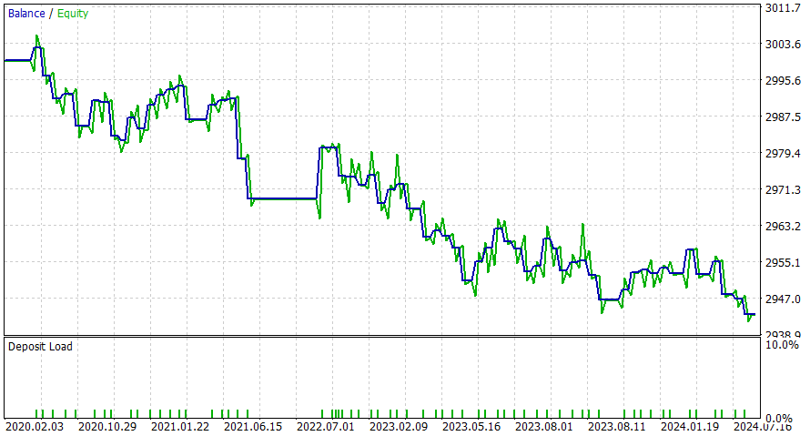

1 hour period of time

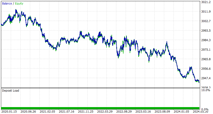
4 hour period of time

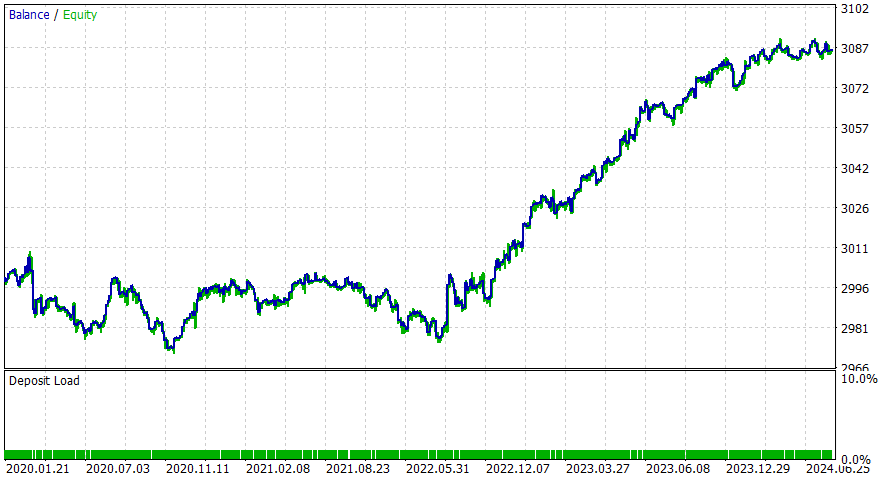
6 hour period of time

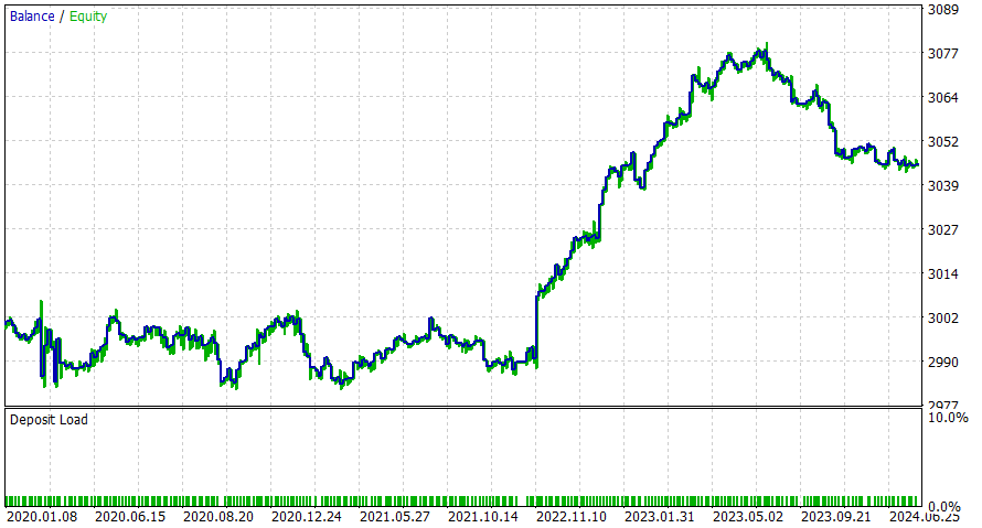
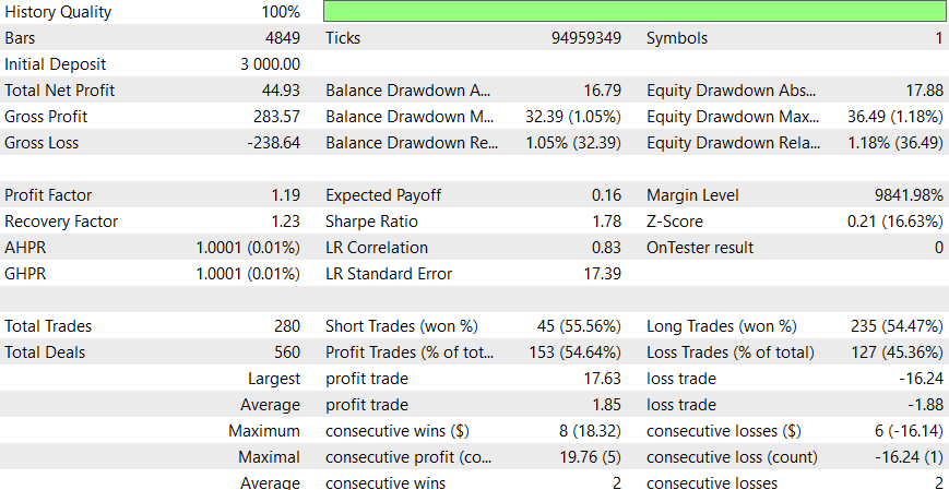
This EA seems to work better during the intraday period, but I am sure you can achieve better results by adding DL or applying the potential improvements consideration.

Conclusion

The SMOC Expert Advisor is a simplified version of a sophisticated approach to automated trading with stochastic modeling and control optimization. Combining several analysis methods, including moving averages, RSI, ATR and custom optimal control algorithms, it aims to make informed trading decisions. The adaptive nature of the system, with features such as dynamic lot sizing and drawdown-based risk adjustment, shows a focus on long-term sustainability. However, as with any trading system, thorough backtesting and forward testing will be critical to assess its real-world performance and reliability.

Farewell: This is just a simple example of an advanced advisor.