
Self Optimizing Expert Advisor With MQL5 And Python (Part V): Deep Markov Models

In our previous discussion on Markov Chains, linked here, we demonstrated how to use a transition matrix to understand the probabilistic behavior of the market. Our transition matrix summarized a lot of information for us. It not only guided us on when to buy and sell, it also informed us whether our market had strong trends or was mostly mean reverting. In today's discussion, we shall change our definition of the system state from the moving averages we used in our first discussion to the Relative Strength Indicator (RSI) indicator instead.
When most people are taught how to trade using the RSI, they are told to buy whenever the RSI reaches 30 and sell when it reaches 70. Some members of the community may question if this is the best decision to make across all markets. We all know that one cannot simply trade all markets the same. This article will demonstrate to you, how you can build your own Markov Chains to algorithmically learn optimal trading rules. Not only that, but the rules that we will learn, dynamically adjust themselves to the data you collect from the market you intend to trade.
Overview of The Trading Strategy
The RSI is widely used by technical analysts to identify extreme price levels. Typically, market prices tend to revert to their averages. Therefore, whenever price analysts find a security hovering in extreme RSI levels, they would normally bet against the dominant trend. This strategy has been slightly altered into many different versions, that all stem from one source. The shortcoming of this strategy is that, what may be considered a strong RSI level in one market, is not necessarily a strong RSI level for all markets.
To illustrate this point, Fig 1 below shows us how the standard deviation of the RSI value evolves on 2 different markets. The Blue line represents the average standard deviation of the RSI in XPDUSD market, while the Orange line represents the NZDJPY market. It is widely known, by all seasoned traders, that the precious metals market is significantly volatile. Therefore, we can see a clear disparity between the changes in RSI levels between the two markets. What may be considered a high reading for the RSI on a currency pair, such as the NZDUSD pair, may be considered ordinary market noise when trading a more volatile instrument, such as the XPDUSD.
It soon becomes apparent that each market could have its own unique level of interest on the RSI indicator. In other words, when we are using the RSI indicator, the optimal level to enter a trade depends on the symbol being traded. Therefore, how can we algorithmically learn on which RSI level should we buy or sell? We can employ our transition matrix to answer this question for any symbol we have in mind.
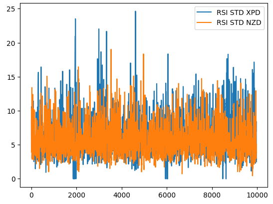
Fig 1: The rolling volatility of the RSI indicator on the XPDUSD Market in blue and the NZDUSD Market in orange
Overview of The Methodology
To learn our strategy from the data we have, we first collected 300 000 rows of M1 data using the MetaTrader 5 library for Python. We labeled the data and then partitioned it into train and test splits. On the training set, we grouped the RSI readings into 10 bins, from 0-10, 11-20, linearly until 91-100. We recorded how price behaved in the future, as it passed through each group on the RSI. The training data showed that price levels had the highest tendency of appreciating whenever price passed through 41-50 zone of the RSI and the highest tendency to depreciate through the 61-70 zone.
We used this estimated transition matrix to build a greedy model that always selected the most probable outcome from the prior distributions. Our simple model scored 52% accuracy on the test set. Another advantage of this approach is its interoperability, we can easily understand how our model is making its decisions. Furthermore, it is now common for AI models being used in important industries to be explainable, and you can rest assured that this family of probabilistic models will not give you compliance issues.
Moving on, our interest was not entirely in the accuracy of the model. Rather, we were invested in the individual accuracy levels of the 10 zones we identified in our training set. Neither of the 2 zones, that had the highest distributions in our training set, proved reliable in the validation set. On the validation set of the data, we obtained the highest accuracy when we bought in 11-20 range, and sold in the 71-80 range. We had accuracy levels of 51.4% and 75.8% from the respective zones. We selected these zones as our optimal zones for opening buy and sell positions on the NZDJPY pair.
Finally, we then set out to build an MQL5 Expert Advisor, that implemented the results of our analysis in Python. Furthermore, we implemented 2 ways of closing positions in our application. We gave the user the decision of either closing positions when the RSI crosses over to a zone that will diminish our open positions, or alternatively, they could close positions whenever price crossed over the moving average.
Fetching And Cleaning The Data
Let us get started, import the libraries we need.
#Let's get started
import MetaTrader5       as mt5
import pandas            as pd
import numpy             as np
import seaborn           as sns
import matplotlib.pyplot as plt
import pandas_ta         as ta
Check if the Terminal can be reached.
mt5.initialize()
Define a few global variables.
#Fetch market data
SYMBOL    = "NZDJPY"
TIMEFRAME = mt5.TIMEFRAME_M1
Let's copy the data from our terminal.
data = pd.DataFrame(mt5.copy_rates_from_pos(SYMBOL,TIMEFRAME,0,300000))
Convert the time format from seconds.
data["time"] = pd.to_datetime(data["time"],unit='s')
Calculate the RSI.
data.ta.rsi(length=20,append=True) Define how far into the future we should forecast.
#Define the look ahead
look_ahead = 20
Label the data.
#Label the data
data["Target"] = np.nan

data.loc[data["close"] > data["close"].shift(-20),"Target"] = -1
data.loc[data["close"] < data["close"].shift(-20),"Target"] = 1
Drop all missing rows from the data.
data.dropna(inplace=True)
data.reset_index(inplace=True,drop=True)
Create a vector to represent the 10 groups of RSI values.
#Create a dataframe
rsi_matrix = pd.DataFrame(columns=["0-10","11-20","21-30","31-40","41-50","51-60","61-70","71-80","81-90","91-100"],index=[0])
This is what our data looks like so far.
data
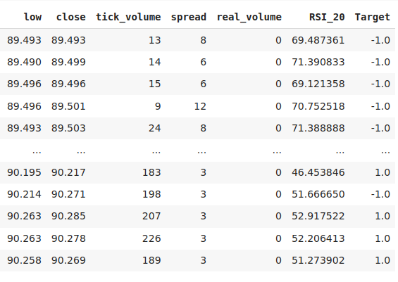
Fig 2: Some of the columns in our data-frame
Initialize the RSI matrix to all 0.
#Initialize the rsi matrix to 0
for i in np.arange(0,9):
    rsi_matrix.iloc[0,i] = 0
Partition the data.
#Split the data into train and test sets
train = data.loc[:(data.shape[0]//2),:]
test  = data.loc[(data.shape[0]//2):,:]
Now we shall go through the training data set and observe each RSI reading, and the corresponding future change in price levels. If the RSI reading was 11, and price levels appreciated 20 steps in the future, we will increment the corresponding 11-20 column in our RSI matrix by one. Furthermore, each time price levels fall, we will penalize the column and decrement it by one. Intuitively, we quickly understand that after in the end, any column with a positive value, corresponds to an RSI level that had a tendency to preceded increasing price levels and the opposite is true for columns that will have negative values.
for i in np.arange(0,train.shape[0]):
    #Fill in the rsi matrix, what happened in the future when we saw RSI readings below 10?
    if((train.loc[i,"RSI_20"] <= 10)):
        rsi_matrix.iloc[0,0] = rsi_matrix.iloc[0,0] + train.loc[i,"Target"]
    #What tends to happen in the future, after seeing RSI readings between 11 and 20?
    if((train.loc[i,"RSI_20"] > 10) & (train.loc[i,"RSI_20"] <= 20)):
        rsi_matrix.iloc[0,1] = rsi_matrix.iloc[0,1] + train.loc[i,"Target"]
    #What tends to happen in the future, after seeing RSI readings between 21 and 30?
    if((train.loc[i,"RSI_20"] > 20) & (train.loc[i,"RSI_20"] <= 30)):
        rsi_matrix.iloc[0,2] = rsi_matrix.iloc[0,2] + train.loc[i,"Target"]
    #What tends to happen in the future, after seeing RSI readings between 31 and 40?
    if((train.loc[i,"RSI_20"] > 30) & (train.loc[i,"RSI_20"] <= 40)):
        rsi_matrix.iloc[0,3] = rsi_matrix.iloc[0,3] + train.loc[i,"Target"]
    #What tends to happen in the future, after seeing RSI readings between 41 and 50?
    if((train.loc[i,"RSI_20"] > 40) & (train.loc[i,"RSI_20"] <= 50)):
        rsi_matrix.iloc[0,4] = rsi_matrix.iloc[0,4] + train.loc[i,"Target"]
    #What tends to happen in the future, after seeing RSI readings between 51 and 60?
    if((train.loc[i,"RSI_20"] > 50) & (train.loc[i,"RSI_20"] <= 60)):
        rsi_matrix.iloc[0,5] = rsi_matrix.iloc[0,5] + train.loc[i,"Target"]
    #What tends to happen in the future, after seeing RSI readings between 61 and 70?
    if((train.loc[i,"RSI_20"] > 60) & (train.loc[i,"RSI_20"] <= 70)):
        rsi_matrix.iloc[0,6] = rsi_matrix.iloc[0,6] + train.loc[i,"Target"]
    #What tends to happen in the future, after seeing RSI readings between 71 and 80?
    if((train.loc[i,"RSI_20"] > 70) & (train.loc[i,"RSI_20"] <= 80)):
        rsi_matrix.iloc[0,7] = rsi_matrix.iloc[0,7] + train.loc[i,"Target"]
    #What tends to happen in the future, after seeing RSI readings between 81 and 90?
    if((train.loc[i,"RSI_20"] > 80) & (train.loc[i,"RSI_20"] <= 90)):
        rsi_matrix.iloc[0,8] = rsi_matrix.iloc[0,8] + train.loc[i,"Target"]
    #What tends to happen in the future, after seeing RSI readings between 91 and 100?
    if((train.loc[i,"RSI_20"] > 90) & (train.loc[i,"RSI_20"] <= 100)):
        rsi_matrix.iloc[0,9] = rsi_matrix.iloc[0,9] + train.loc[i,"Target"]
This is the distribution of counts in the training set. We have arrived at our first problem, there were no training observations in the 91-100 zone. Therefore, I decided to assume that since the neighboring zones all resulted in falling price levels, we will assign the zone an arbitrary negative value.
rsi_matrix
| 0-10 | 11-20 | 21-30 | 31-40 | 41-50 | 51-60 | 61-70 | 71-80 | 81-90 | 91-100 |
|---|---|---|---|---|---|---|---|---|---|
| 4.0 | 47.0 | 221.0 | 1171.0 | 3786.0 | 945.0 | -1159.0 | -35.0 | -3.0 | NaN |
We can visualize this distribution. It appears that price spends most of its time in the 31-70 zone. This corresponds to the middle part of the RSI. As we mentioned earlier, price appeared to be very bullish in the 41-50 region, and bearish in the 61-70 region. However, these appeared to be just artifacts of the training data because this relationship did not hold true on the validation data.
sns.barplot(rsi_matrix)
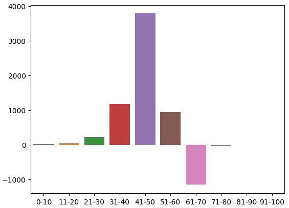
Fig 3: The distribution of the observed effects of the RSI zones
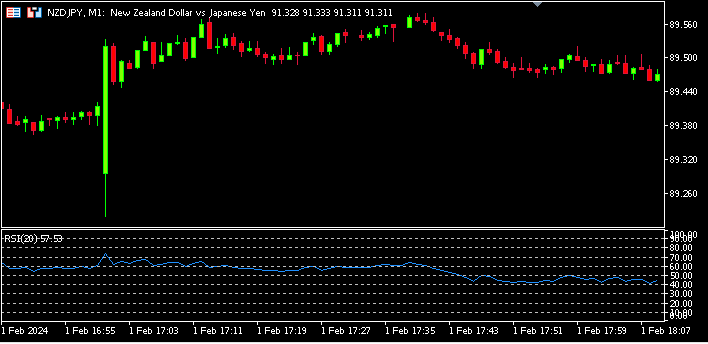
Fig 4: A visual representation of our transformations so far
Now we shall evaluate our model's accuracy on validation data. First, reset the index of the training data.
test.reset_index(inplace=True,drop=True)
Create a column for our model's predictions.
test["Predictions"] = np.nan Fill in our model's predictions.
for i in np.arange(0,test.shape[0]):
    #Fill in the predictions
    if((test.loc[i,"RSI_20"] <= 10)):
        test.loc[i,"Predictions"] = 1

    if((test.loc[i,"RSI_20"] > 10) & (test.loc[i,"RSI_20"] <= 20)):
        test.loc[i,"Predictions"] = 1

    if((test.loc[i,"RSI_20"] > 20) & (test.loc[i,"RSI_20"] <= 30)):
        test.loc[i,"Predictions"] = 1

    if((test.loc[i,"RSI_20"] > 30) & (test.loc[i,"RSI_20"] <= 40)):
        test.loc[i,"Predictions"] = 1

    if((test.loc[i,"RSI_20"] > 40) & (test.loc[i,"RSI_20"] <= 50)):
        test.loc[i,"Predictions"] = 1

    if((test.loc[i,"RSI_20"] > 50) & (test.loc[i,"RSI_20"] <= 60)):
        test.loc[i,"Predictions"] = 1

    if((test.loc[i,"RSI_20"] > 60) & (test.loc[i,"RSI_20"] <= 70)):
        test.loc[i,"Predictions"] = -1

    if((test.loc[i,"RSI_20"] > 70) & (test.loc[i,"RSI_20"] <= 80)):
        test.loc[i,"Predictions"] = -1

    if((test.loc[i,"RSI_20"] > 80) & (test.loc[i,"RSI_20"] <= 90)):
        test.loc[i,"Predictions"] = -1

    if((test.loc[i,"RSI_20"] > 90) & (test.loc[i,"RSI_20"] <= 100)):
        test.loc[i,"Predictions"] = -1
Validate we do not have any null values.
test.loc[:,"Predictions"].isna().any() Let us describe the relationship between our model's predictions and the target, using pandas. The most common entry is True, this is a good indicator.
(test["Target"] == test["Predictions"]).describe()
unique 2
top True
freq 77409
dtype: object
Let us estimate how accurate our model is.
#Our estimation of the model's accuracy
((test["Target"] == test["Predictions"]).describe().freq / (test["Target"] == test["Predictions"]).shape[0])
We are interested in the accuracy of each of the 10 RSI zones.
val_err = []
Record our accuracy in each zone.
val_err.append(test.loc[(test["RSI_20"] < 10) & (test["Predictions"] == test["Target"])].shape[0] / test.loc[test["RSI_20"] < 10].shape[0])
val_err.append(test.loc[((test["RSI_20"] <= 20) & (test["RSI_20"] > 10)) & (test["Predictions"] == test["Target"])].shape[0] / test.loc[((test["RSI_20"] <= 20) & (test["RSI_20"] > 10))].shape[0])
val_err.append(test.loc[((test["RSI_20"] <= 30) & (test["RSI_20"] > 20)) & (test["Predictions"] == test["Target"])].shape[0] / test.loc[((test["RSI_20"] <= 30) & (test["RSI_20"] > 20))].shape[0])
val_err.append(test.loc[((test["RSI_20"] <= 40) & (test["RSI_20"] > 30)) & (test["Predictions"] == test["Target"])].shape[0] / test.loc[((test["RSI_20"] <= 40) & (test["RSI_20"] > 30))].shape[0])
val_err.append(test.loc[((test["RSI_20"] <= 50) & (test["RSI_20"] > 40)) & (test["Predictions"] == test["Target"])].shape[0] / test.loc[((test["RSI_20"] <= 50) & (test["RSI_20"] > 40))].shape[0])
val_err.append(test.loc[((test["RSI_20"] <= 60) & (test["RSI_20"] > 50)) & (test["Predictions"] == test["Target"])].shape[0] / test.loc[((test["RSI_20"] <= 60) & (test["RSI_20"] > 50))].shape[0])
val_err.append(test.loc[((test["RSI_20"] <= 70) & (test["RSI_20"] > 60)) & (test["Predictions"] == test["Target"])].shape[0] / test.loc[((test["RSI_20"] <= 70) & (test["RSI_20"] > 60))].shape[0])
val_err.append(test.loc[((test["RSI_20"] <= 80) & (test["RSI_20"] > 70)) & (test["Predictions"] == test["Target"])].shape[0] / test.loc[((test["RSI_20"] <= 80) & (test["RSI_20"] > 70))].shape[0])
val_err.append(test.loc[((test["RSI_20"] <= 90) & (test["RSI_20"] > 80)) & (test["Predictions"] == test["Target"])].shape[0] / test.loc[((test["RSI_20"] <= 90) & (test["RSI_20"] > 80))].shape[0])
val_err.append(test.loc[((test["RSI_20"] <= 100) & (test["RSI_20"] > 90)) & (test["Predictions"] == test["Target"])].shape[0] / test.loc[((test["RSI_20"] <= 100) & (test["RSI_20"] > 90))].shape[0])
Plotting our accuracy. The red line is our 50% cut off point, any RSI zone beneath this line may not be reliable. We can clearly observe that the last zone has a perfect score of 1. However, recall that this corresponds to the missing 91-100 zone that did not occur once in more than 100 000 minutes of training data we had. Therefore, this zone is probably rare to see and not optimal for our trading requirement. The 11-20 zone has accuracy levels of 75%, the highest from our bullish zones. The same was true for the 71-80 zone, it had the highest accuracy among all the bearish zones.
plt.plot(val_err)
plt.plot(fifty,'r') 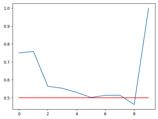
FIg 5: Visualizing our validation accuracy
Our validation accuracy across the different RSI zones. Notice that we obtained 100% accuracy in the 91-100 range. Recall that our training set was approximately 100 000 rows, but we did not observe any RSI readings in that zone. Therefore, we can conclude price rarely reaches those extremes so that result may not be an optimal decision for us.
| 0-10 | 11-20 | 21-30 | 31-40 | 41-50 | 51-60 | 61-70 | 71-80 | 81-90 | 91-100 |
|---|---|---|---|---|---|---|---|---|---|
| 0.75 | 0.75 | 0.56 | 0.55 | 0.53 | 0.50 | 0.51 | 0.51 | 0.46 | 1.0 |
Building Our Deep Markov Model
So far, we have only built a model that learns from the past distribution of data. Could it be possible for us to enhance this strategy by stacking a more flexible learner, to learn an optimal strategy of using our Markov Model? Let's train a deep neural network and give it the predictions made by the Markov Model as inputs, and the observed changes in price levels will be the target. To accomplish this task effectively, we will need to subdivide our training set to 2 halves. We will fit our new Markov Model using just the first half of the training set. Our neural network will be fit on the Markov Model's predictions on the first half training set, and the corresponding changes in price levels.
We observed that both our neural network and our simple Markov model out performed an identical neural network attempting to learn changes to price levels directly from the OHLC market quotes. These conclusions were drawn from our test data that had not been used in the training procedure. Astonishingly, our deep neural network and our Simple Markov model performed on par. Therefore, this may be seen as a call for greater effort, to outperform the benchmark set by the Markov Model.
Let us get started by importing the libraries we need.
#Let us now try find a machine learning model to learn how to optimally use our transition matrix
from sklearn.neural_network import MLPClassifier
from sklearn.metrics import accuracy_score
from sklearn.model_selection import train_test_split,TimeSeriesSplit
Now, we need to perform a train test split, on our training data.
#Now let us partition our train set into 2 halves
train , train_val = train_test_split(train,shuffle=False,test_size=0.5)
Fit the Markov model on the new train set.
#Now let us recalculate our transition matrix, based on the first half of the training set
rsi_matrix.iloc[0,0] = train.loc[(train["RSI_20"] < 10) & (train["Target"] == 1)].shape[0] / train.loc[(train["RSI_20"] < 10)].shape[0]
rsi_matrix.iloc[0,1] = train.loc[((train["RSI_20"] > 10) & (train["RSI_20"] <=20)) & (train["Target"] == 1)].shape[0] / train.loc[((train["RSI_20"] > 10) & (train["RSI_20"] <=20))].shape[0]
rsi_matrix.iloc[0,2] = train.loc[((train["RSI_20"] > 20) & (train["RSI_20"] <=30)) & (train["Target"] == 1)].shape[0] / train.loc[((train["RSI_20"] > 20) & (train["RSI_20"] <=30))].shape[0]
rsi_matrix.iloc[0,3] = train.loc[((train["RSI_20"] > 30) & (train["RSI_20"] <=40)) & (train["Target"] == 1)].shape[0] / train.loc[((train["RSI_20"] > 30) & (train["RSI_20"] <=40))].shape[0]
rsi_matrix.iloc[0,4] = train.loc[((train["RSI_20"] > 40) & (train["RSI_20"] <=50)) & (train["Target"] == 1)].shape[0] / train.loc[((train["RSI_20"] > 40) & (train["RSI_20"] <=50))].shape[0]
rsi_matrix.iloc[0,5] = train.loc[((train["RSI_20"] > 50) & (train["RSI_20"] <=60)) & (train["Target"] == 1)].shape[0] / train.loc[((train["RSI_20"] > 50) & (train["RSI_20"] <=60))].shape[0]
rsi_matrix.iloc[0,6] = train.loc[((train["RSI_20"] > 60) & (train["RSI_20"] <=70)) & (train["Target"] == 1)].shape[0] / train.loc[((train["RSI_20"] > 60) & (train["RSI_20"] <=70))].shape[0]
rsi_matrix.iloc[0,7] = train.loc[((train["RSI_20"] > 70) & (train["RSI_20"] <=80)) & (train["Target"] == 1)].shape[0] / train.loc[((train["RSI_20"] > 70) & (train["RSI_20"] <=80))].shape[0]
rsi_matrix.iloc[0,8] = train.loc[((train["RSI_20"] > 80) & (train["RSI_20"] <=90)) & (train["Target"] == 1)].shape[0] / train.loc[((train["RSI_20"] > 80) & (train["RSI_20"] <=90))].shape[0]

rsi_matrix
| 0-10 | 11-20 | 21-30 | 31-40 | 41-50 | 51-60 | 61-70 | 71-80 | 81-90 | 91-100 |
|---|---|---|---|---|---|---|---|---|---|
| 1.0 | 0.655172 | 0.541701 | 0.536398 | 0.53243 | 0.516551 | 0.460306 | 0.491154 | 0.395349 | 0 |
We can visualize this probability distribution. Recall that these quantities represent the probability of price levels rising 20 minutes into the future, after the price has passed through each of the 10 RSI zones. The red line represents the 50% level. All zones above the 50% level are bullish, and all zones beneath are bearish. This is what we can assume to be true, given the first half of the training data.
#From the training set, it appears that RSI readings above 61 are bearish and RSI readings below 61 are bullish
plt.plot(rsi_matrix.iloc[0,:])
plt.plot(fifty,'r')
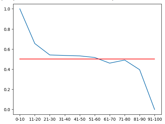
Fig 6: From the first half of the training set, it appears all zones beneath 61 are bullish, and above 61 are bearish
Recording the new predictions made by the Markov model.
#Let's now store our model's predictions
train["Predictions"] = -1
train.loc[train["RSI_20"] < 61,"Predictions"] = 1

train_val["Predictions"] = -1
train_val.loc[train_val["RSI_20"] < 61,"Predictions"] = 1

test["Predictions"] = -1
test.loc[test["RSI_20"] < 61,"Predictions"] = 1
Before we can start using neural networks, as a rule of thumb, standardizing and scaling helps. Furthermore, our RSI is on a fixed scale from 0-100 while our price readings are without bounds. In such cases, standardization is necessary.
#Let's Standardize and scale our data
from sklearn.preprocessing import RobustScaler
Define our inputs and target.
ohlc_predictors = ["open","high","low","close","tick_volume","spread","RSI_20"]
transition_matrix = ["Predictions"]
all_predictors = ohlc_predictors + transition_matrix
target = ["Target"]
Scale the data.
scaler = RobustScaler()
scaler =  scaler.fit(train.loc[:,predictors])
train_scaled = pd.DataFrame(scaler.transform(train.loc[:,predictors]),columns=predictors)
train_val_scaled = pd.DataFrame(scaler.transform(train_val.loc[:,predictors]),columns=predictors)
test_scaled = pd.DataFrame(scaler.transform(test.loc[:,predictors]),columns=predictors)
Create data-frames to store our accuracy.
#Create a dataframe to store our cv error on the training set, validation training set and the test set
train_err     = pd.DataFrame(columns=["Transition Matrix","Deep Markov Model","OHLC Model","All Model"],index=np.arange(0,5))
train_val_err = pd.DataFrame(columns=["Transition Matrix","Deep Markov Model","OHLC Model","All Model"],index=[0])
test_err      = pd.DataFrame(columns=["Transition Matrix","Deep Markov Model","OHLC Model","All Model"],index=[0])
Define the time-series split object.
#Create a time series split object
tscv = TimeSeriesSplit(n_splits = 5,gap=look_ahead)
Cross validate the models.
model = MLPClassifier(hidden_layer_sizes=(20,10))
for i , (train_index,test_index) in enumerate(tscv.split(train_scaled)):
    #Fit the model
    model.fit(train.loc[train_index,transition_matrix],train.loc[train_index,"Target"])
    #Record its accuracy
    train_err.iloc[i,1] = accuracy_score(train.loc[test_index,"Target"],model.predict(train.loc[test_index,transition_matrix]))

#Record our accuracy levels on the validation training set
train_val_err.iloc[0,1] = accuracy_score(train_val.loc[:,"Target"],model.predict(train_val.loc[:,transition_matrix]))

#Record our accuracy levels on the test set
test_err.iloc[0,1] = accuracy_score(test.loc[:,"Target"],model.predict(test.loc[:,transition_matrix]))

#Our accuracy levels on the training set
train_err
Let us now observe our model's accuracy on the validation half of the training set.
train_val_err.iloc[0,0] = train_val.loc[train_val["Predictions"] == train_val["Target"]].shape[0] / train_val.shape[0]
train_val_err
| Transition Matrix | Deep Markov Model | OHLC Model | All Model |
|---|---|---|---|
| 0.52309 | 0.52309 | 0.507306 | 0.517291 |
Now, most importantly, let us see our accuracy on the test data set. As we can see from the two tables, our hybrid Deep Markov Model failed to outperform our simple Markov Model. In my opinion, this took me by surprise. It could possibly imply that our procedure for training the Deep Neural Network was not optimal, alternatively we can always search over a broader pool of candidate machine learning models. Another interesting attribute of our results is that, the model that used all the data didn't perform best.
The good news is that we managed to outperform the benchmark set by trying to predict price directly from the market quotes. It appears that the Markov Model's simple heuristics, help the neural network quickly learn lower level market structure.
test_err.iloc[0,0] = test.loc[test["Predictions"] == test["Target"]].shape[0] / test.shape[0]
test_err
| Transition Matrix | Deep Markov Model | OHLC Model | All Model |
|---|---|---|---|
| 0.519322 | 0.519322 | 0.497127 | 0.496724 |
Implementing in MQL5
To implement our RSI based Expert Advisor, we will start by first importing the libraries we need.
//+------------------------------------------------------------------+
//|                                                     Auto RSI.mq5 |
//|                                        Gamuchirai Zororo Ndawana |
//|                          https://www.mql5.com/en/gamuchiraindawa |
//+------------------------------------------------------------------+
#property copyright "Gamuchirai Zororo Ndawana"
#property link      "https://www.mql5.com/en/gamuchiraindawa"
#property version   "1.00"

//+------------------------------------------------------------------+
//| Libraries                                                        |
//+------------------------------------------------------------------+
#include <Trade\Trade.mqh>
CTrade Trade;
Now let us define our global variables.
//+------------------------------------------------------------------+
//| Global variables                                                 |
//+------------------------------------------------------------------+
int rsi_handler;
double rsi_buffer[];
int ma_handler;
int system_state;
double ma_buffer[];
double bid,ask;

//--- Custom enumeration
enum close_conditions
  {
   MA_Close  = 0,
   RSI_Close
  };
We need to obtain inputs from our user.
//+------------------------------------------------------------------+
//| Inputs                                                           |
//+------------------------------------------------------------------+
input group "Technical Indicators"
input int rsi_period = 20; //RSI Period
input int ma_period = 20; //MA Period

input group "Money Management"
input double trading_volume = 0.3; //Lot size

input group "Trading Rules"
input close_conditions user_close = RSI_Close; //How should we close the positions?
Whenever our Expert Advisor is loaded for the first time, let us load the indicators and validate them.
//+------------------------------------------------------------------+
//| Expert initialization function                                   |
//+------------------------------------------------------------------+
int OnInit()
  {
//--- Load the indicator
   rsi_handler = iRSI(_Symbol,PERIOD_M1,rsi_period,PRICE_CLOSE);
   ma_handler = iMA(_Symbol,PERIOD_M1,ma_period,0,MODE_EMA,PRICE_CLOSE);

//--- Validate our technical indicators
   if(rsi_handler == INVALID_HANDLE || ma_handler == INVALID_HANDLE)
     {
      //--- We failed to load the rsi
      Comment("Failed to load the RSI Indicator");
      return(INIT_FAILED);
     }

//---
   return(INIT_SUCCEEDED);
  }
If our application is not in use, release the indicators.
//+------------------------------------------------------------------+
//| Expert deinitialization function                                 |
//+------------------------------------------------------------------+
void OnDeinit(const int reason)
  {
//--- Release our technical indicators
   IndicatorRelease(rsi_handler);
   IndicatorRelease(ma_handler);
  }
Finally, we have no open positions, use our follow our model's trading rules. Otherwise, if we do have an open position, follow the user's instructions on how to close the trades.
//+------------------------------------------------------------------+
//| Expert tick function                                             |
//+------------------------------------------------------------------+
void OnTick()
  {
//--- Update market and technical data
   update();

//--- Check if we have any open positions
   if(PositionsTotal() == 0)
     {
      check_setup();
     }

   if(PositionsTotal() > 0)
     {
      manage_setup();
     }
  }
//+------------------------------------------------------------------+
The following function will close our positions depending on whether the user wants us to use the trading rules we have learned from the RSI or the simple moving average. If the use wants us to use the moving average, we will simply close our positions whenever price crosses over the moving average.
//+------------------------------------------------------------------+
//| Manage our open setups                                           |
//+------------------------------------------------------------------+
void manage_setup(void)
  {
   if(user_close == RSI_Close)
     {
      if((system_state == 1) && ((rsi_buffer[0] > 71) && (rsi_buffer[80] <= 80)))
        {
         PositionSelect(Symbol());
         Trade.PositionClose(PositionGetTicket(0));
         return;
        }

      if((system_state == -1) && ((rsi_buffer[0] > 11) && (rsi_buffer[80] <= 20)))
        {
         PositionSelect(Symbol());
         Trade.PositionClose(PositionGetTicket(0));
         return;
        }
     }


   else
      if(user_close == MA_Close)
        {
         if((iClose(_Symbol,PERIOD_CURRENT,0) > ma_buffer[0]) && (system_state == -1))
           {
            PositionSelect(Symbol());
            Trade.PositionClose(PositionGetTicket(0));
            return;
           }

         if((iClose(_Symbol,PERIOD_CURRENT,0) < ma_buffer[0]) && (system_state == 1))
           {
            PositionSelect(Symbol());
            Trade.PositionClose(PositionGetTicket(0));
            return;
           }
        }
  }
The following function, will check if we have any valid setups. That is, if price has entered any of our profitable zones. Furthermore, if the user has specified that we should use the moving average to close our positions, then we will wait for price to be on the right side of the moving average first before we decide whether we should open a position.
//+------------------------------------------------------------------+
//| Find if we have any setups to trade                              |
//+------------------------------------------------------------------+
void check_setup(void)
  {

   if(user_close == RSI_Close)
     {
      if((rsi_buffer[0] > 71) && (rsi_buffer[0] <= 80))
        {
         Trade.Sell(trading_volume,_Symbol,bid,0,0,"Auto RSI");
         system_state = -1;
        }

      if((rsi_buffer[0] > 11) && (rsi_buffer[0] <= 20))
        {
         Trade.Buy(trading_volume,_Symbol,ask,0,0,"Auto RSI");
         system_state = 1;
        }
     }

   if(user_close == MA_Close)
     {
      if(((rsi_buffer[0] > 71) && (rsi_buffer[0] <= 80)) && (iClose(_Symbol,PERIOD_CURRENT,0) < ma_buffer[0]))
        {
         Trade.Sell(trading_volume,_Symbol,bid,0,0,"Auto RSI");
         system_state = -1;
        }

      if(((rsi_buffer[0] > 11) && (rsi_buffer[0] <= 20)) && (iClose(_Symbol,PERIOD_CURRENT,0) > ma_buffer[0]))
        {
         Trade.Buy(trading_volume,_Symbol,ask,0,0,"Auto RSI");
         system_state = 1;
        }
     }
  }
This function will update our technical and market data.
//+------------------------------------------------------------------+
//| Fetch market quotes and technical data                           |
//+------------------------------------------------------------------+
void update(void)
  {
   bid = SymbolInfoDouble(_Symbol,SYMBOL_BID);
   ask = SymbolInfoDouble(_Symbol,SYMBOL_ASK);

   CopyBuffer(rsi_handler,0,0,1,rsi_buffer);
   CopyBuffer(ma_handler,0,0,1,ma_buffer);
  }
//+------------------------------------------------------------------+
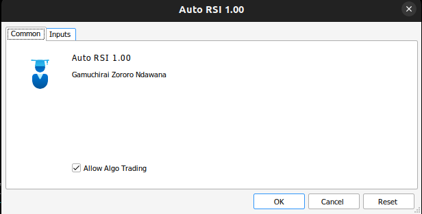
Fig 7: Our Expert Advisor
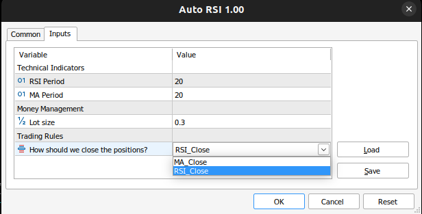
Fig 8: Our Expert Advisor Application
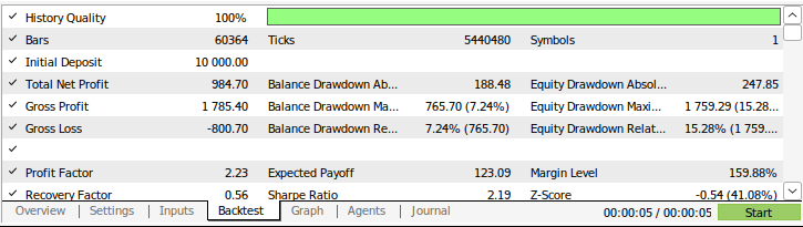
Fig 9: The results of back-testing our strategy
Conclusion
In this article, we have demonstrated the power of simple probabilistic models. To our surprise, we could not outperform the simple Markov model by trying to learn from its mistakes. However, if you have been following this article series closely, then you will probably share my viewpoint that we are now heading in the right direction. We are slowly accumulating a set of algorithms that are easier to model than price itself, under the constraints of being just as informative as modelling price itself. Join us in our next discussions as we will try to learn why it will take to outperform the simple Markov Model.
Warning: All rights to these materials are reserved by MetaQuotes Ltd. Copying or reprinting of these materials in whole or in part is prohibited.
This article was written by a user of the site and reflects their personal views. MetaQuotes Ltd is not responsible for the accuracy of the information presented, nor for any consequences resulting from the use of the solutions, strategies or recommendations described.

- Free trading apps
- Over 8,000 signals for copying
- Economic news for exploring financial markets
You agree to website policy and terms of use
Thanks for your efforts , It is helpful to have the video as well . please note your link to the previous article comes up with a 404 for me
Sorry for the dead link, it slipped past me, my mistake there.