
Reimagining Classic Strategies (Part X): Can AI Power The MACD?

The moving average cross-over is probably one of the oldest existing trading strategies. The Moving Average Convergence Divergence (MACD) is a very popular indicator is built on top of the notion of moving average cross-overs. There are many new members of our community who may be curious to know the predictive power of the MACD indicator, in their search to build the best trading strategy possible. Additionally, there are seasoned technical analysts who utilize the MACD in their strategies who may hold the same question in mind. This article will present you with an empirical analysis of the indicator's predictive power on the EURUSD pair. Additionally, we will equip you with modelling techniques you can use to enhance your technical analysis with AI.
Overview of The Trading Strategy
The MACD indicator is primarily used to identify market trends and measure trend momentum. The indicator was created in the 1970s by the late Gerrald Appel. Appel was a money manager for his private clients, and his success was rooted in his technical analysis approach to trading. He invented the MACD indicator approximately 50 years ago.

Fig 1: Gerald Appel creator of the MACD indicator
Technical analysts employ the indicator to identify entry and exit points in various ways. Fig 2 below is a screenshot of the MACD indicator applied to the GBPUSD pair using its default settings. The indicator is included into your installation of MetaTrader 5 by default. The red line, called the MACD main, is calculated by the difference between two moving averages, one fast and the other slow. Whenever the main line crosses beneath 0, the market is most likely in a downtrend, and the opposite is true when the line crosses above 0.
Like wise, the main line itself can also be used to identify market strength. Only appreciating price levels, will cause the value of the main line to increase, and conversely depreciating price levels will cause the main line to fall. Therefore, the turning points, where the main line forms a shape resembling a cup, are created by a shift in the market's momentum. Various trading strategies have been implemented around the MACD. More elaborate and sophisticated strategies seek to identify MACD divergence.
MACD divergence occurs when price levels rally in a strong trend, breaking to new extreme levels. Whilst on the other hand, the MACD indicator is in a trend that only grows shallower and begins falling in sharp contrast to strong price action seen on the chart. Typically, MACD divergence is interpreted as an early warning of trend reversal, allowing traders to roll back their open positions before the markets become more volatile.
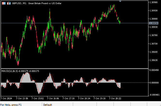
Fig 2: The MACD indicator with its default settings on the GBPUSD M1 chart
There are many skeptics that question the use of the MACD indicator all together. Let us start by addressing the elephant in the room. All technical indicators are grouped as lagging indicators. That means, technical indicators only change after price levels change, they cannot change before price levels. Macroeconomic indicators such as global inflation levels and geopolitical news such as the outbreak of war or a natural disaster may offset supply and demand levels. They are considered leading indicators because they can quickly change before price levels reflect that change.
Many traders hold the opinion that these lagged signals will most likely cause traders to enter their positions when the market move has already been exhausted. Furthermore, it is commonplace to observe trend reversals that were not preceded by MACD divergences. And to the same effect, it is also possible to observe MACD divergence that was not followed by a trend reversal.
These facts call us to question the reliability of the indicator, and whether it truly has any predictive power worthy of merit. We desire to assess if it is possible to overcome the inherent lag of the indicator using AI. If the MACD indicator turns out to be resilient, we will integrate an AI model that either:
- Uses the indicator values to forecast future price levels.
- Forecasts the MACD indicator itself.
Depending on which modelling approach renders lower error. Otherwise, if our analysis suggests that the MACD may not have predictive power under our current strategy, we will instead opt for the best performing model when forecasting price levels.
Overview of The Methodology
Our analysis began with a customized script written in MQL5 to fetch exactly 100 000 rows of M1 market quotes on the EURUSD and their corresponding MACD signal and main values into a CSV file. Judging by our data visualizations, the MACD indicator appears to be a poor separator of future price levels. The changes in price levels are most likely independent of the indicator's value, additionally, the indicator's calculation gave the data a non-linear and complex structure that may be challenging to model.
The data we obtained from our MetaTrader 5 terminal was partitioned into 2 halves. We used the first half to estimate our model's accuracy using 5-fold cross validation. We subsequently created 3 identical Deep Neural Network models and trained them on 3 different subsets of our data:
- Price model: Forecast price levels using OHLC market quotes from MetaTrader 5
- MACD model: Forecast MACD indicator values using OHLC quotes and the MACD reading
- Complete model: Forecast price levels using OHLC quotes and the MACD indicator
The latter half of the partition was used to test the models. The first model scored the highest accuracy on the test, 69%. Our feature selection algorithms suggested that the market quotes we obtained from MetaTrader 5 were more informative than the MACD values.
Thus, we began optimizing the best model we had, a regression model forecasting the future price of the EURUSD pair. However, we quickly ran into problems because our learned the noise in our training data. We dismally failed to outperform a simple linear regression on the test set. Therefore, we substituted the over optimized model for a Support Vector Machine (SVM) instead.
We subsequently exported our SVM model into ONNX format, and built an expert advisor using a combined approach of forecasting future EURUSD price levels and the MACD indicator.
Fetching The Data We Need
To get the ball rolling, our first stop was the MetaEditor Integrated Development Environment (IDE). We created the script outlined below to fetch our market data from the MetaTrader 5 terminal. We requested 100 000 rows of historical M1 data and exported it to CSV format. The script below will fill our CSV file with the Time, Open, High, Low, Close and the 2 MACD values. Simply drag and drop the script onto any pair you wish to analyze, if you wish to follow along with us.
//+------------------------------------------------------------------+
//|                                                      ProjectName |
//|                                      Copyright 2020, CompanyName |
//|                                       http://www.companyname.net |
//+------------------------------------------------------------------+
#property copyright "Gamuchirai Zororo Ndawana"
#property link      "https://www.mql5.com/en/users/gamuchiraindawa"
#property version   "1.00"
#property script_show_inputs

//+------------------------------------------------------------------+
//| Script Inputs                                                    |
//+------------------------------------------------------------------+
input int size = 100000; //How much data should we fetch?

//+------------------------------------------------------------------+
//| Global variables                                                 |
//+------------------------------------------------------------------+
int indicator_handler;
double indicator_buffer[];
double indicator_buffer_2[];

//+------------------------------------------------------------------+
//| On start function                                                |
//+------------------------------------------------------------------+
void OnStart()
  {

//--- Load indicator
   indicator_handler = iMACD(Symbol(),PERIOD_CURRENT,12,26,9,PRICE_CLOSE);
   CopyBuffer(indicator_handler,0,0,size,indicator_buffer);
   CopyBuffer(indicator_handler,1,0,size,indicator_buffer_2);
   ArraySetAsSeries(indicator_buffer,true);
   ArraySetAsSeries(indicator_buffer_2,true);

//--- File name
   string file_name = "Market Data " + Symbol() +" MACD " +  ".csv";

//--- Write to file
   int file_handle=FileOpen(file_name,FILE_WRITE|FILE_ANSI|FILE_CSV,",");

   for(int i= size;i>=0;i--)
     {
      if(i == size)
        {
         FileWrite(file_handle,"Time","Open","High","Low","Close","MACD Main","MACD Signal");
        }

      else
        {
         FileWrite(file_handle,iTime(Symbol(),PERIOD_CURRENT,i),
                   iOpen(Symbol(),PERIOD_CURRENT,i),
                   iHigh(Symbol(),PERIOD_CURRENT,i),
                   iLow(Symbol(),PERIOD_CURRENT,i),
                   iClose(Symbol(),PERIOD_CURRENT,i),
                   indicator_buffer[i],
                   indicator_buffer_2[i]
                  );
        }
     }
//--- Close the file
   FileClose(file_handle);
  }
//+------------------------------------------------------------------+
Data Preprocessing
Now that we have exported our data into CSV format, let us read in the data in our Python workspace. First, we shall load the libraries we need.
#Load libraries
import pandas as pd
import numpy as np
import seaborn as sns
import matplotlib.pyplot as plt
Read in the data.
#Read in the data
data = pd.read_csv("Market Data EURUSD MACD .csv")
Define how far into the future we should forecast.
#Forecast horizon
look_ahead = 20
Let us add binary targets to flag if the current reading is greater than the previous 20 instances before it, for both the EURUSD close price and the MACD main line.
#Let's add labels
data["Bull Bear"] = np.where(data["Close"] < data["Close"].shift(look_ahead),0,1)
data["MACD Bull"] = np.where(data["MACD Main"] < data["MACD Main"].shift(look_ahead),0,1)

data = data.loc[20:,:]

data
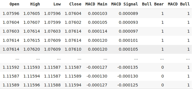
Fig 3: Some of the columns in our data frame
Additionally, we need to define our target values.
data["MACD Target"] = data["MACD Main"].shift(-look_ahead)
data["Price Target"] = data["Close"].shift(-look_ahead)

data["MACD Binary Target"] = np.where(data["MACD Main"] < data["MACD Target"],1,0)
data["Price Binary Target"] = np.where(data["Close"] < data["Price Target"],1,0)

data = data.iloc[:-20,:]
Exploratory Data Analysis
Scatter plots help us visualize the relationship between a dependent and independent variable. The plot below shows us there is definitely a relationship between future price levels and the current MACD reading, the challenge is that the relationship is non-linear and appears to have a complex structure. It is not immediately obvious as to what changes in the MACD indicator result in bullish or bearish price performance.
sns.scatterplot(data=data,x="MACD Main",y="MACD Signal",hue="Price Binary Target")
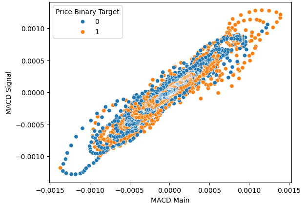
Fig 4: Visualizing the relationship between the MACD indicator and price levels
Performing a 3D plot only further demonstrates how convoluted the relationship truly is. There are no defined boundaries, so we would expect the data to be challenging to classify. The only intelligent deductions we can draw from our plot is that the markets appears to quickly cluster back towards the center after passing through extreme levels on the MACD.
#Define the 3D Plot
fig = plt.figure(figsize=(7,7))
ax = plt.axes(projection="3d")
ax.scatter(data["MACD Main"],data["MACD Signal"],data["Close"],c=data["Price Binary Target"])
ax.set_xlabel("MACD Main")
ax.set_ylabel("MACD Signal")
ax.set_zlabel("EURUSD Close")
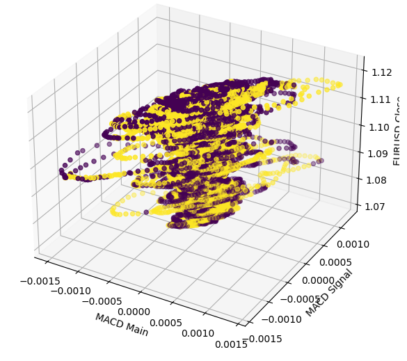
Fig 5: Visualizing the interaction between the MACD indicator and the EURUSD market
Violin plots allow us to, simultaneously, visualize the distribution of data and compare 2 distributions. The blue outline represents a summary of the observed distribution of future price levels after the MACD has risen or fallen. In Fig 6 below, we wanted to understand if the rising or falling of the MACD indicator is associated with different distributions regarding future price movements. As we can see, the 2 distributions appear almost identical. Furthermore, the core of each distribution has box plot. The mean values of both box plots appear almost the same, regardless of whether the indicator was in a bullish or bearish state.
sns.violinplot(data=data,x="MACD Bull",y="Close",hue="Price Binary Target",split=True,fill=False)
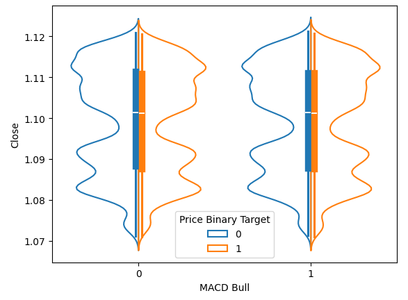
Fig 6: Visualizing the effect of the MACD indicator on future price levels
Preparing To Model The Data
Let us now get started modelling our data, first and foremost we need to import our libraries.
#Perform train test splits
from sklearn.model_selection import train_test_split,TimeSeriesSplit
from sklearn.metrics import accuracy_score
train,test = train_test_split(data,test_size=0.5,shuffle=False)
Now we shall define the predictors and target.
#Let's scale the data
ohlc_predictors = ["Open","High","Low","Close","Bull Bear"]
macd_predictors = ["MACD Main","MACD Signal","MACD Bull"]
all_predictors  = ohlc_predictors + macd_predictors
cv_predictors   = [ohlc_predictors,macd_predictors,all_predictors]

#Define the targets
cv_targets = ["MACD Binary Target","Price Binary Target","All"]
Scaling the data.
#Scaling the data
from sklearn.preprocessing import MinMaxScaler
scaler = MinMaxScaler()
scaler.fit(train[all_predictors])
train_scaled = pd.DataFrame(scaler.transform(train[all_predictors]),columns=all_predictors)
test_scaled = pd.DataFrame(scaler.transform(test[all_predictors]),columns=all_predictors)
Let us load the libraries we need.
#Import the models we will evaluate
from sklearn.neural_network import MLPClassifier,MLPRegressor
from sklearn.linear_model import LinearRegression
Create the time series split object.
tscv = TimeSeriesSplit(n_splits=5,gap=look_ahead) The indexes of our data frame will map to the set of inputs we were evaluating.
err_indexes = ["MACD Train","Price Train","All Train","MACD Test","Price Test","All Test"]
Now we will create the data frame that will record our estimations of the model's accuracy as we change our inputs.
#Now let us define a table to store our error levels
columns = ["Model Accuracy"]

cv_err = pd.DataFrame(columns=columns,index=err_indexes)
Reset all our indexes.
#Reset index
train = train.reset_index(drop=True)
test = test.reset_index(drop=True)
Let us cross validate the model. We will cross validate the model on the training set, and then record its accuracy on the test set without fitting it to the test set.
#Initailize the model
price_model = MLPClassifier(hidden_layer_sizes=(10,6))
macd_model  = MLPClassifier(hidden_layer_sizes=(10,6))
all_model   = MLPClassifier(hidden_layer_sizes=(10,6))

price_acc = []
macd_acc = []
all_acc = []

#Cross validate each model twice
for j,(train_index,test_index) in enumerate(tscv.split(train_scaled)):
  #Fit the models
  price_model.fit(train_scaled.loc[train_index,ohlc_predictors],train.loc[train_index,"Price Binary Target"])
  macd_model.fit(train_scaled.loc[train_index,all_predictors],train.loc[train_index,"MACD Binary Target"])
  all_model.fit(train_scaled.loc[train_index,all_predictors],train.loc[train_index,"Price Binary Target"])
  #Store the accuracy
  price_acc.append(accuracy_score(train.loc[test_index,"Price Binary Target"],price_model.predict(train_scaled.loc[test_index,ohlc_predictors])))
  macd_acc.append(accuracy_score(train.loc[test_index,cv_targets[0]],macd_model.predict(train_scaled.loc[test_index,all_predictors])))
  all_acc.append(accuracy_score(train.loc[test_index,cv_targets[1]],all_model.predict(train_scaled.loc[test_index,all_predictors])))

#Now we can store our estimates of the model's error
cv_err.iloc[0,0] = np.mean(price_acc)
cv_err.iloc[1,0] = np.mean(macd_acc)
cv_err.iloc[2,0] = np.mean(all_acc)
#Estimating test error
cv_err.iloc[3,0] = accuracy_score(test[cv_targets[1]],price_model.predict(test_scaled[ohlc_predictors]))
cv_err.iloc[4,0] = accuracy_score(test[cv_targets[0]],macd_model.predict(test_scaled[all_predictors]))
cv_err.iloc[5,0] = accuracy_score(test[cv_targets[1]],all_model.predict(test_scaled[all_predictors]))
| Input Group | Model Accuracy |
|---|---|
| MACD Train | 0.507129 |
| OHLC Train | 0.690267 |
| All Train | 0.504577 |
| MACD Test | 0.48669 |
| OHLC Test | 0.684069 |
| All Test | 0.487442 |
Feature Importance
Let us now try to estimate feature importance levels for our deep neural network. We will select permutation importance to interpret our model. Permutation importance defines the importance of each input by first shuffling the values of that input column and then assessing the changes in model accuracy. The idea is that, important features will cause large drops in error, while unimportant features will cause changes in the model's accuracy that are close to 0.
However, there are considerations to be made. First, the permutation importance algorithm randomly shuffles each of the model's inputs. This means that the algorithm may randomly shuffle the Open price and set it higher than the High price. This is obviously not possible in the real world. Therefore, we should interpret the results of the algorithm with a pinch of salt. One could say the algorithm is biased because it assesses feature importance under simulated conditions that could potentially never happen, needlessly penalizing the model. Additionally, due to the stochastic nature of the optimization algorithms used to fit modern neural networks, training the same neural networks on the same data set could render remarkably different explanations each time.
#Let us try assess feature importance
from sklearn.inspection import permutation_importance
from sklearn.linear_model import RidgeClassifier
We will now fit our permutation importance object on our trained deep neural network model. You have the option of passing the training or test data to be shuffled, we chose the test data. Afterward, we arranged the data by order of drop in accuracy caused and plotted the results. Fig 7 below displays the observed permutation importance scores. We can see the effects of shuffling the inputs related to the MACD appear very close to 0, implying that the MACD columns aren't that important to our model.
#Let us fit the model
model   = MLPClassifier(hidden_layer_sizes=(10,6))
model.fit(train_scaled.loc[:,all_predictors],train.loc[:,"Price Binary Target"])

#Calculate permutation importance scores
pi = permutation_importance(
    model, test_scaled.loc[:,all_predictors], test.loc[:,"Price Binary Target"], n_repeats=10, random_state=42, n_jobs=-1
)

#Sort the importance scores
sorted_importances_idx = pi.importances_mean.argsort()
importances = pd.DataFrame(
    pi.importances[sorted_importances_idx].T,
    columns=test_scaled.columns[sorted_importances_idx],
)

#Create the plot
ax = importances.plot.box(vert=False, whis=10)
ax.set_title("Permutation Importances (test set)")
ax.axvline(x=0, color="k", linestyle="--")
ax.set_xlabel("Decrease in accuracy score")
ax.figure.tight_layout()
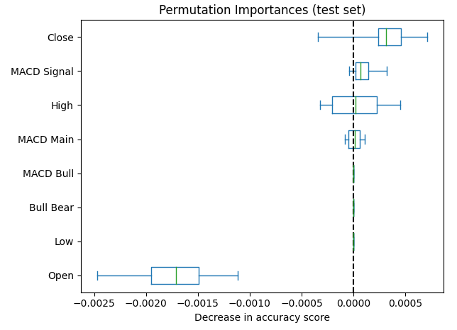
Fig 7: Our permutation importance scores ranked the Close price as the most important feature
Fitting a simpler model could also give us insight into the importance levels of the inputs. The ridge classifier is a linear model that pushes its coefficients closer and closer to 0 in the direction that minimizes its error. Therefore, assuming your data has been standardized and scaled, unimportant features will have the smallest ridge coefficients. If you were curious, the ridge classifier can achieve this by extending the ordinary linear model to include a penalty term proportional to the squared sum of the model coefficients. This is commonly known as L2-regularization.
#Let us fit the model
model   = RidgeClassifier()
model.fit(train_scaled.loc[:,all_predictors],train.loc[:,"Price Binary Target"])
Now let us plot the model's coefficients.
ridge_importance = pd.DataFrame(model.coef_.tolist(),columns=all_predictors)

#Prepare the plot
fig,ax = plt.subplots(figsize=(10,5))
sns.barplot(ridge_importance,ax=ax)
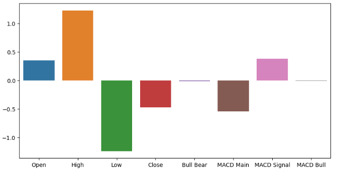
Fig 8: Our ridge coefficients suggest to us that the High and Low price are the most informative features we have
Parameter Tuning
Now we will try to optimize our best performing model. However as we stated earlier, our optimization routine was not successful on this turn. Unfortunately, this is inherent in the nature of optimization algorithms, we are not guaranteed to find solutions. Performing parameter optimization does not necessarily mean the model you obtain at the end will be better, we are only attempting to approximate optimal model parameters. Let us load the libraries we need.
#Let's tune our model further
from sklearn.model_selection import RandomizedSearchCV
Defining the model.
#Reinitialize the model
model  = MLPRegressor(max_iter=200)
Now we will define the tuner object. The object will evaluate our model under different initialization parameters and return an object that contains the best performing inputs found.
#Define the tuner
tuner = RandomizedSearchCV(
        model,
        {
        "activation" : ["relu","logistic","tanh","identity"],
        "solver":["adam","sgd","lbfgs"],
        "alpha":[0.1,0.01,0.001,0.0001,0.00001,0.00001,0.0000001],
        "tol":[0.1,0.01,0.001,0.0001,0.00001,0.000001,0.0000001],
        "learning_rate":['constant','adaptive','invscaling'],
        "learning_rate_init":[0.1,0.01,0.001,0.0001,0.00001,0.000001,0.0000001],
        "hidden_layer_sizes":[(2,4,8,2),(10,20),(5,10),(2,20),(6,8,10),(1,5),(20,10),(8,4),(2,4,8),(10,5)],
        "early_stopping":[True,False],
        "warm_start":[True,False],
        "shuffle": [True,False]
        },
        n_iter=100,
        cv=5,
        n_jobs=-1,
        scoring="neg_mean_squared_error"
)
Fitting the tuner object.
tuner.fit(train.loc[:,ohlc_predictors],train.loc[:,"Price Target"]) The best parameters we found.
tuner.best_params_
'tol': 0.01,
'solver': 'sgd',
'shuffle': False,
'learning_rate_init': 0.01,
'learning_rate': 'constant',
'hidden_layer_sizes': (20, 10),
'early_stopping': True,
'alpha': 1e-07,
'activation': 'identity'}
Deeper Optimization
We can search even deeper for better input settings by employing the SciPy library. We will use the library to estimate the results of global optimization over the model's continuous parameters.#Deeper optimization from scipy.optimize import minimize from sklearn.metrics import mean_squared_error from sklearn.model_selection import TimeSeriesSplit
Define the time-series split object.
#Define the time series split object
tscv = TimeSeriesSplit(n_splits=5,gap=look_ahead)
Create data structures to store our accuracy levels.
#Create a dataframe to store our accuracy
current_error_rate = pd.DataFrame(index = np.arange(0,5),columns=["Current Error"])
algorithm_progress = []
Our cost function to be minimized will be the model's error levels on training data.
#Define the objective function
def objective(x):
    #The parameter x represents a new value for our neural network's settings
    model = MLPRegressor(hidden_layer_sizes=tuner.best_params_["hidden_layer_sizes"],
                         early_stopping=tuner.best_params_["early_stopping"],
                         warm_start=tuner.best_params_["warm_start"],
                         max_iter=500,
                         activation=tuner.best_params_["activation"],
                         learning_rate=tuner.best_params_["learning_rate"],
                         solver=tuner.best_params_["solver"],
                         shuffle=tuner.best_params_["shuffle"],
                         alpha=x[0],
                         tol=x[1],
                         learning_rate_init=x[2]
                         )
    #Now we will cross validate the model
    for i,(train_index,test_index) in enumerate(tscv.split(train)):
        #Train the model
        model.fit(train.loc[train_index,ohlc_predictors],train.loc[train_index,"Price Target"])
        #Measure the RMSE
        current_error_rate.iloc[i,0] = mean_squared_error(train.loc[test_index,"Price Target"],model.predict(train.loc[test_index,ohlc_predictors]))
    #Store the algorithm's progress
    algorithm_progress.append(current_error_rate.iloc[:,0].mean())
    #Return the Mean CV RMSE
    return(current_error_rate.iloc[:,0].mean())
SciPy expects us to supply it with initial values to start the optimization procedure.
#Define the starting point
pt = [tuner.best_params_["alpha"],tuner.best_params_["tol"],tuner.best_params_["learning_rate_init"]]
bnds = ((10.00 ** -100,10.00 ** 100),
        (10.00 ** -100,10.00 ** 100),
        (10.00 ** -100,10.00 ** 100))
Let us now try to optimize the model.
#Searching deeper for parameters
result = minimize(objective,pt,method="L-BFGS-B",bounds=bnds)
It appears the algorithm managed to converge. This means it found stable inputs that had little variance. Therefore, it concluded that there are no better solutions because the changes in error levels were approaching 0.
#The result of our optimization
result success: True
status: 0
fun: 3.730365831424036e-06
x: [ 9.939e-08 9.999e-03 9.999e-03]
nit: 3
jac: [-7.896e+01 -1.133e+02 1.439e+03]
nfev: 100
njev: 25
hess_inv: <3x3 LbfgsInvHessProduct with dtype=float64>
Let us visualize the procedure.
#Store the optimal coefficients
optimal_weights = result.x
optima_y = min(algorithm_progress)
optima_x = algorithm_progress.index(optima_y)
inputs = np.arange(0,len(algorithm_progress))

#Plot the performance of our optimization procedure
plt.scatter(inputs,algorithm_progress)
plt.plot(optima_x,optima_y,'ro',color='r')
plt.axvline(x=optima_x,ls='--',color='red')
plt.axhline(y=optima_y,ls='--',color='red')
plt.xlabel("Iterations")
plt.ylabel("Training MSE")
plt.title("Minimizing Training Error")
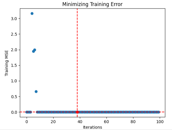
Fig 9: Visualizing the optimization of a Deep Neural Network
Testing For Over-fitting
Over-fitting is an undesired effect whereby our model learns meaningless representations from the data we gave it. It is undesired because a model in this state will render poor accuracy levels. We can tell if our model is over-fitting by comparing it against weaker learners, and default instances of a similar neural network. If our model is learning the noise and failing to pick up the signal in the data, it will be outperformed by the weaker learners. However, even if our model outperforms the weaker learners, there's still a chance its over-fitting.
#Testing for overfitting
#Benchmark
benchmark = LinearRegression()

#Default
default_nn = MLPRegressor(max_iter=500)

#Randomized NN
random_search_nn = MLPRegressor(hidden_layer_sizes=tuner.best_params_["hidden_layer_sizes"],
                         early_stopping=tuner.best_params_["early_stopping"],
                         warm_start=tuner.best_params_["warm_start"],
                         max_iter=500,
                         activation=tuner.best_params_["activation"],
                         learning_rate=tuner.best_params_["learning_rate"],
                         solver=tuner.best_params_["solver"],
                         shuffle=tuner.best_params_["shuffle"],
                         alpha=tuner.best_params_["alpha"],
                         tol=tuner.best_params_["tol"],
                         learning_rate_init=tuner.best_params_["learning_rate_init"]
                         )

#LBFGS NN
lbfgs_nn = MLPRegressor(hidden_layer_sizes=tuner.best_params_["hidden_layer_sizes"],
                         early_stopping=tuner.best_params_["early_stopping"],
                         warm_start=tuner.best_params_["warm_start"],
                         max_iter=500,
                         activation=tuner.best_params_["activation"],
                         learning_rate=tuner.best_params_["learning_rate"],
                         solver=tuner.best_params_["solver"],
                         shuffle=tuner.best_params_["shuffle"],
                         alpha=result.x[0],
                         tol=result.x[1],
                         learning_rate_init=result.x[2]
                         )
Fit the models and asses their accuracy. We can clearly see a disparity in performance, the linear regression model out classed all our deep neural networks. I decided to then try fitting a linear SVM instead. It performed better than the neural networks did, but failed to outperform the linear regression.
#Fit the models on the training sets
benchmark = LinearRegression()
benchmark.fit(((train.loc[:,ohlc_predictors])),train.loc[:,"Price Target"])
mean_squared_error(test.loc[:,"Price Target"],benchmark.predict(((test.loc[:,ohlc_predictors]))))

#Test the default
default_nn.fit(train.loc[:,ohlc_predictors],train.loc[:,"Price Target"])
mean_squared_error(test.loc[:,"Price Target"],default_nn.predict(test.loc[:,ohlc_predictors]))

#Test the random search
random_search_nn.fit(train.loc[:,ohlc_predictors],train.loc[:,"Price Target"])
mean_squared_error(test.loc[:,"Price Target"],random_search_nn.predict(test.loc[:,ohlc_predictors]))

#Test the lbfgs nn
lbfgs_nn.fit(train.loc[:,ohlc_predictors],train.loc[:,"Price Target"])
mean_squared_error(test.loc[:,"Price Target"],lbfgs_nn.predict(test.loc[:,ohlc_predictors])
| Linear Regression | Default NN | Random Search | LBFGS NN |
|---|---|---|---|
| 2.609826e-07 | 1.996431e-05 | 0.00051 | 0.000398 |
Let us fit our LinearSVR, it is more likely to pick up the non-linear interactions in our data.
#From experience, I'll try LSVR
from sklearn.svm import LinearSVR
Initialize the model and fit it on all the data we have. Observe the SVR's error levels are better than the neural network, but not as good as the linear regression.
#Initialize the model
lsvr = LinearSVR()

#Fit the Linear Support Vector
lsvr.fit(train.loc[:,["Open","High","Low","Close"]],train.loc[:,"Price Target"])
mean_squared_error(test.loc[:,"Price Target"],lsvr.predict(test.loc[:,["Open","High","Low","Close"]]))
Exporting To ONNX
Open Neural Network Exchange (ONNX), allows us to create machine learning models in one language and then share them to any other language that supports the ONNX API. The ONNX protocol is rapidly changing the number of environments under which machine learning can be leveraged. ONNX allows us to seamlessly integrate AI into our MQL5 Expert Advisor.
#Let's export the LSVR to ONNX
import onnx
from skl2onnx import convert_sklearn
from skl2onnx.common.data_types import FloatTensorType
Create a new instance of the model.
model = LinearSVR()
Fit the model on all the data we have.
model.fit(data.loc[:,["Open","High","Low","Close"]],data.loc[:,"Price Target"])
Define the model's input shape.
#Define the input type
initial_types = [("float_input",FloatTensorType([1,4]))]
Create an ONNX representation of the model.
#Create the ONNX representation
onnx_model = convert_sklearn(model,initial_types=initial_types,target_opset=12)
Save the ONNX model.
# Save the ONNX model
onnx.save_model(onnx_model,"EURUSD SVR M1.onnx")

Fig 10:Visualizing our ONNX model
Implementing in MQL5
We can now begin implementing our strategy in MQL5. We want to build an application that buys whenever price is above the moving average and the AI predicts prices will appreciate.
To get started with our application, we will first include the ONNX file we just created into our Expert Advisor.
//+--------------------------------------------------------------+
//| EURUSD AI                                                    |
//+--------------------------------------------------------------+
#property copyright "Gamuchirai Ndawana"
#property link "https://metaquotes.com/en/users/gamuchiraindawa"
#property version "2.1"
#property description "Supports M1"

//+--------------------------------------------------------------+
//| Resources we need                                            |
//+--------------------------------------------------------------+
#resource "\\Files\\EURUSD SVR M1.onnx" as const uchar onnx_buffer[];
Now we shall load the trade library.
//+--------------------------------------------------------------+
//| Libraries                                                    |
//+--------------------------------------------------------------+
#include  <Trade\Trade.mqh>
CTrade trade;
Define a few constants that will now change.
//+--------------------------------------------------------------+
//| Constants                                                    |
//+--------------------------------------------------------------+
const double  stop_percent = 1;
const int     ma_period_shift = 0;
We will allow the user control over the technical indicators parameters, and the general behavior of the program.
//+--------------------------------------------------------------+
//| User inputs                                                  |
//+--------------------------------------------------------------+
input group "TAs"
input double atr_multiple =2.5;             //How wide should the stop loss be?
input int    atr_period = 200;              //ATR Period
input int    ma_period = 1000;              //Moving average period

input group "Risk"
input double risk_percentage= 0.02;         //Risk percentage (0.01 - 1)
input double profit_target = 1.0;           //Profit target
Let us now define all the global variables we need.
//+--------------------------------------------------------------+
//| Global variables                                             |
//+--------------------------------------------------------------+
double position_size = 2;
int lot_multiplier = 1;
bool  buy_break_even_setup = false;
bool  sell_break_even_setup = false;
double up_level = 0.03;
double down_level = -0.03;
double min_volume,max_volume_increase, volume_step, buy_stop_loss, sell_stop_loss,ask, bid,atr_stop,mid_point,risk_equity;
double take_profit = 0;
double close_price[3];
double moving_average_low_array[],close_average_reading[],moving_average_high_array[],atr_reading[];
long   min_distance,login;
int    ma_high,ma_low,atr,close_average;
bool   authorized = false;
double tick_value,average_market_move,margin,mid_point_height,channel_width,lot_step;
string currency,server;
bool all_closed =true;
long onnx_model;
vectorf onnx_output = vectorf::Zeros(1);
ENUM_ACCOUNT_TRADE_MODE account_type;
Our expert will first check that the user has enabled Experts to trade the account, then it will attempt to load the ONNX model, and finally if successful so far, we will then load our technical indicators.
//+------------------------------------------------------------------+
//| On initialization                                                |
//+------------------------------------------------------------------+
int OnInit()
  {

//--- Authorization
   if(!auth())
     {
      return(INIT_FAILED);
     }

//--- Load the ONNX model
if(!load_onnx())
   {
      return(INIT_FAILED);
   }

//--- Everything went fine
   else
     {
      load();
      return(INIT_SUCCEEDED);
     }
  }
If our Advisor is not in use, we will free up the memory allocated to the ONNX model.
//+------------------------------------------------------------------+
//| On deinitialization                                              |
//+------------------------------------------------------------------+
void OnDeinit(const int reason)
  {
      OnnxRelease(onnx_model);
  }
Whenever we receive updated price feeds, we will update our global market variables and then check for trading signals if we have no open positions. Otherwise, we will update our trailing stop loss.
//+------------------------------------------------------------------+
//| On every tick                                                    |
//+------------------------------------------------------------------+
void OnTick()
  {
//On Every Function Call
   update();
   static datetime time_stamp;
   datetime time = iTime(_Symbol,PERIOD_CURRENT,0);
   Comment("AI Forecast: ",onnx_output[0]);

//On Every Candle
   if(time_stamp != time)
     {

      //Mark the candle
      time_stamp = time;

      OrderCalcMargin(ORDER_TYPE_BUY,_Symbol,min_volume,ask,margin);
      calculate_lot_size();
      if(PositionsTotal() == 0)
        {
         check_signal();
        }
     }

//--- If we have positions, manage them.
   if(PositionsTotal() > 0)
     {
      check_atr_stop();
      check_profit();
     }
  }


//+------------------------------------------------------------------+
//| Check if we have any valid setups, and execute them              |
//+------------------------------------------------------------------+
void check_signal(void)
  {
  //--- Get a prediction from our model
  model_predict();
     if(onnx_output[0] > iClose(Symbol(),PERIOD_CURRENT,0))
      {
         if(above_channel())
           {
               check_buy();
           }
      }

      else
         if(below_channel())
           {
             if(onnx_output[0] < iClose(Symbol(),PERIOD_CURRENT,0))
               {
                  check_sell();
                }
           }
  }
This function is responsible for updating all our global market variables.
//+------------------------------------------------------------------+
//| Update our global variables                                      |
//+------------------------------------------------------------------+
void update(void)
  {
//--- Important details that need to be updated everytick
   ask = SymbolInfoDouble(_Symbol,SYMBOL_ASK);
   bid = SymbolInfoDouble(_Symbol,SYMBOL_BID);
   buy_stop_loss = 0;
   sell_stop_loss = 0;
   check_price(3);
   CopyBuffer(ma_high,0,0,1,moving_average_high_array);
   CopyBuffer(ma_low,0,0,1,moving_average_low_array);
   CopyBuffer(atr,0,0,1,atr_reading);
   ArraySetAsSeries(moving_average_high_array,true);
   ArraySetAsSeries(moving_average_low_array,true);
   ArraySetAsSeries(atr_reading,true);
   risk_equity = AccountInfoDouble(ACCOUNT_BALANCE) * risk_percentage;
   atr_stop = (((min_distance + (atr_reading[0]* 1e5) * atr_multiple) * _Point));
   mid_point = (moving_average_high_array[0] + moving_average_low_array[0]) / 2;
   mid_point_height = close_price[0] - mid_point;
   channel_width = moving_average_high_array[0] - moving_average_low_array[0];
  }
Now we must define the function that will ensure our application is allowed to run, if it isn't allowed to run, the function will give the user instructions on what to do, and return false which will halt initialization.
//+------------------------------------------------------------------+
//| Check if the EA is allowed to be run                             |
//+------------------------------------------------------------------+
bool auth(void)
  {
   if(!TerminalInfoInteger(TERMINAL_TRADE_ALLOWED))
     {
      Comment("Press Ctrl + E To Give The Robot Permission To Trade And Reload The Program");
      return(false);
     }

   else
      if(!MQLInfoInteger(MQL_TRADE_ALLOWED))
        {
         Comment("Reload The Program And Make Sure You Clicked Allow Algo Trading");
         return(false);
        }

   return(true);
  }
During initialization, we need a function responsible for loading all our technical indicators and fetching important market details. The load function will do just that for us and since it is referencing global variables, its return type will be void.
//+---------------------------------------------------------------------+
//| Load our needed variables                                           |
//+---------------------------------------------------------------------+
void load(void)
  {
//Account Info
   currency = AccountInfoString(ACCOUNT_CURRENCY);
   server = AccountInfoString(ACCOUNT_SERVER);
   login = AccountInfoInteger(ACCOUNT_LOGIN);

//Indicators
   atr = iATR(_Symbol,PERIOD_CURRENT,atr_period);
   ma_high = iMA(_Symbol,PERIOD_CURRENT,ma_period,ma_period_shift,MODE_EMA,PRICE_HIGH);
   ma_low = iMA(_Symbol,PERIOD_CURRENT,ma_period,ma_period_shift,MODE_EMA,PRICE_LOW);

//Market Information
   min_volume = SymbolInfoDouble(_Symbol,SYMBOL_VOLUME_MIN);
   max_volume_increase = SymbolInfoDouble(_Symbol,SYMBOL_VOLUME_MAX) / SymbolInfoDouble(_Symbol,SYMBOL_VOLUME_MIN);
   min_distance = SymbolInfoInteger(_Symbol,SYMBOL_TRADE_STOPS_LEVEL);
   tick_value = SymbolInfoDouble(_Symbol,SYMBOL_TRADE_TICK_VALUE_PROFIT) * min_volume;
   lot_step = SymbolInfoDouble(_Symbol,SYMBOL_VOLUME_STEP);
   average_market_move = NormalizeDouble(10000 * tick_value,_Digits);
  }
Our ONNX model on the other hand, will be loaded by a separate function call. The function will create our ONNX model from the buffer we defined earlier and validate the input and output shape.
//+------------------------------------------------------------------+
//| Load our ONNX model                                              |
//+------------------------------------------------------------------+
bool load_onnx(void)
   {
      onnx_model = OnnxCreateFromBuffer(onnx_buffer,ONNX_DEFAULT);
      ulong onnx_input [] = {1,4};
      ulong onnx_output[] = {1,1};
      if(!OnnxSetInputShape(onnx_model,0,onnx_input))
         {
            Comment("[INTERNAL ERROR] Failed to load AI modules. Relode the EA.");
            return(false);
         }

      if(!OnnxSetOutputShape(onnx_model,0,onnx_output))
         {
            Comment("[INTERNAL ERROR] Failed to load AI modules. Relode the EA.");
            return(false);
         }

     return(true);
   }
Let us now define the function that will get predictions from our model.
//+------------------------------------------------------------------+
//| Get a prediction from our model                                  |
//+------------------------------------------------------------------+
void model_predict(void)
   {
      vectorf onnx_inputs = {iOpen(Symbol(),PERIOD_CURRENT,0),iHigh(Symbol(),PERIOD_CURRENT,0),iLow(Symbol(),PERIOD_CURRENT,0),iClose(Symbol(),PERIOD_CURRENT,0)};
      OnnxRun(onnx_model,ONNX_DEFAULT,onnx_inputs,onnx_output);
   }
Our stop loss will be adjusted by the ATR value. Depending on whether the current trade is a buy or a sell trade, that is the main determining factor that helps us know if we should update our stop loss up, by adding the current ATR value, or down, by subtracting the current ATR value. We can also use a multiple of the current ATR value, to give the user finer grain control over their risk levels.
//+------------------------------------------------------------------+
//| Update the ATR stop loss                                         |
//+------------------------------------------------------------------+
void check_atr_stop()
  {

   for(int i = PositionsTotal() -1; i >= 0; i--)
     {

      string symbol = PositionGetSymbol(i);
      if(_Symbol == symbol)
        {

         ulong ticket = PositionGetInteger(POSITION_TICKET);
         double position_price = PositionGetDouble(POSITION_PRICE_OPEN);
         double type = PositionGetInteger(POSITION_TYPE);
         double current_stop_loss = PositionGetDouble(POSITION_SL);

         if(type == POSITION_TYPE_BUY)
           {
            double atr_stop_loss = (ask - (atr_stop));
            double atr_take_profit = (ask + (atr_stop));

            if((current_stop_loss < atr_stop_loss) || (current_stop_loss == 0))
              {
               trade.PositionModify(ticket,atr_stop_loss,atr_take_profit);
              }
           }

         else
            if(type == POSITION_TYPE_SELL)
              {
               double atr_stop_loss = (bid + (atr_stop));
               double atr_take_profit = (bid - (atr_stop));
               if((current_stop_loss > atr_stop_loss) || (current_stop_loss == 0))
                 {
                  trade.PositionModify(ticket,atr_stop_loss,atr_take_profit);
                 }
              }
        }
     }
  }
Lastly we need to define 2 functions responsible for opening buy and sell positions, and their complementary pairs for closing the position.
//+------------------------------------------------------------------+
//| Open buy positions                                               |
//+------------------------------------------------------------------+
void check_buy()
  {
   if(PositionsTotal() == 0)
     {
      for(int i=0; i < position_size;i++)
        {
         trade.Buy(min_volume * lot_multiplier,_Symbol,ask,buy_stop_loss,0,"BUY");
         Print("Position: ",i," has been setup");
        }
     }
  }

//+------------------------------------------------------------------+
//| Open sell positions                                              |
//+------------------------------------------------------------------+
void check_sell()
  {
   if(PositionsTotal() == 0)
     {
      for(int i=0; i < position_size;i++)
        {
         trade.Sell(min_volume * lot_multiplier,_Symbol,bid,sell_stop_loss,0,"SELL");
         Print("Position: ",i," has been setup");
        }
     }
  }

//+------------------------------------------------------------------+
//| Close all buy positions                                          |
//+------------------------------------------------------------------+
void close_buy()
  {
   ulong ticket;
   int type;
   if(PositionsTotal() > 0)
     {
      for(int i = 0; i < PositionsTotal();i++)
        {
         if(PositionGetSymbol(i) == _Symbol)
           {
            ticket = PositionGetTicket(i);
            type = (int)PositionGetInteger(POSITION_TYPE);
            if(type == POSITION_TYPE_BUY)
              {
               trade.PositionClose(ticket);
              }
           }
        }
     }
  }

//+------------------------------------------------------------------+
//| Close all sell positions                                         |
//+------------------------------------------------------------------+
void close_sell()
  {
   ulong ticket;
   int type;
   if(PositionsTotal() > 0)
     {
      for(int i = 0; i < PositionsTotal();i++)
        {
         if(PositionGetSymbol(i) == _Symbol)
           {
            ticket = PositionGetTicket(i);
            type = (int)PositionGetInteger(POSITION_TYPE);
            if(type == POSITION_TYPE_SELL)
              {
               trade.PositionClose(ticket);
              }
           }
        }
     }
  }
Let us keep track of the last 3 price levels.
//+------------------------------------------------------------------+
//| Get the last 3 quotes                                            |
//+------------------------------------------------------------------+
void check_price(int candles)
  {
   for(int i = 0; i < candles;i++)
     {
      close_price[i] = iClose(_Symbol,PERIOD_CURRENT,i);
     }
  }
This boolean check will return true if we are above the moving average.
//+------------------------------------------------------------------+
//| Are we completely above the MA?                                  |
//+------------------------------------------------------------------+
bool above_channel()
  {
   return (((close_price[0] - moving_average_high_array[0] > 0)) && ((close_price[0] - moving_average_low_array[0]) > 0));
  }
Check if we are below the moving average.
//+------------------------------------------------------------------+
//| Are we completely below the MA?                                  |
//+------------------------------------------------------------------+
bool below_channel()
  {
   return(((close_price[0] - moving_average_high_array[0]) < 0) && ((close_price[0] - moving_average_low_array[0]) < 0));
  }
Close all the positions we have.
//+------------------------------------------------------------------+
//| Close all positions we have                                      |
//+------------------------------------------------------------------+
void close_all()
  {
   if(PositionsTotal() > 0)
     {
      ulong ticket;
      for(int i =0;i < PositionsTotal();i++)
        {
         ticket = PositionGetTicket(i);
         trade.PositionClose(ticket);
        }
     }
  }
Calculate the optimal lot size to use so that our margin is equal to the amount of capital we are willing to risk.
//+------------------------------------------------------------------+
//| Calculate the lot size to be used                                |
//+------------------------------------------------------------------+
void calculate_lot_size()
  {
//--- This is the total percentage of the account we're willing to part with for margin, or to keep a position open in other words.
   Print("Risk Equity: ",risk_equity);

//--- Now that we're ready to part with a discrete amount for margin, how many positions can we afford under the current lot size?
//--- By default we always start from minimum lot
   position_size = risk_equity / margin;

//--- We need to keep the number of positions lower than 10
   if(position_size > 10)
     {
      //--- How many times is it greater than 10?
      int estimated_lot_size = (int)  MathFloor(position_size / 10);
      position_size = risk_equity / (margin * estimated_lot_size);
      Print("Position Size After Dividing By margin at new estimated lot size: ",position_size);
      int estimated_position_size = position_size;
      //--- Can we increase the lot size this many times?
      if(estimated_lot_size < max_volume_increase)
        {
         Print("Est Lot Size: ",estimated_lot_size," Position Size: ",estimated_position_size);
         lot_multiplier = estimated_lot_size;
         position_size = estimated_position_size;
        }
     }
  }
Close open positions, and check if we can trade again.
//--- This function will help us keep track of which side we need to enter the market
void close_all_and_enter()
  {

   if(PositionSelect(Symbol()))
     {
      // Determine the type of position
      check_signal();
     }
   else
     {
      Print("No open position found.");
     }
  }
If we have reached our profit target, close all the positions we have to realize the profit, and then check if we can enter again.
//+------------------------------------------------------------------+
//| Chekc if we have reached our profit target                       |
//+------------------------------------------------------------------+
void check_profit()
  {
   double current_profit = (AccountInfoDouble(ACCOUNT_EQUITY) - AccountInfoDouble(ACCOUNT_BALANCE)) / PositionsTotal();
   if(current_profit > profit_target)
     {
      close_all_and_enter();
     }

   if((current_profit * PositionsTotal()) < (risk_equity * -1))
     {
      Comment("We've breached our risk equity, consider closing all positions");
     }
  }
Lastly, we need a function that will close all our unprofitable trades.
//+------------------------------------------------------------------+
//| Close all losing trades                                          |
//+------------------------------------------------------------------+
void close_profitable_trades()
  {
   for(int i=PositionsTotal()-1; i>=0; i--)
     {
      if(PositionSelectByTicket(PositionGetTicket(i)))
        {
         if(PositionGetDouble(POSITION_PROFIT)>profit_target)
           {
            ulong ticket;
            ticket = PositionGetTicket(i);
            trade.PositionClose(ticket);
           }
        }
     }
  }
//+------------------------------------------------------------------+
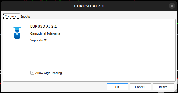
Fig 11: Our Expert Advisor
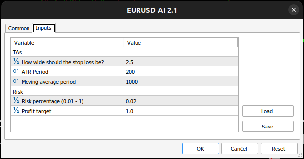
Fig 12: The parameters we are using to test the application
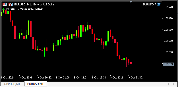
Fig 13: Our application in action
Conclusion
While our results were not encouraging, they are far from conclusive. There are other ways of interpreting the MACD indicator that may be worth an evaluation. For example, during a bull trend the MACD signal line crosses above the main line, and it falls beneath the main line in a bear trend. Viewing the indicator from this perspective could yield different error metrics. We cannot simply assume that all strategies of interpreting the MACD will yield uniform error levels. It would only be reasonable for us to sample the effectiveness of different strategies based on the MACD before we can gather an opinion of the indicator's effectiveness.
 Body in Connexus (Part 4): Adding HTTP body support
- Free trading apps
- Over 8,000 signals for copying
- Economic news for exploring financial markets
You agree to website policy and terms of use