Reimagining Classic Strategies (Part IX): Multiple Time Frame Analysis (II)

MetaTrader 5 — Examples | 9 October 2024, 08:55

237

There are many time-frames for traders to use. For a new member of the community, or anyone who may be learning how to trade, the choice can be difficult to make. Even seasoned traders frequently debate and share different viewpoints, trying to establish just which time-frame is optimal. We will attempt to answer this question objectively, by defining the optimal time frame as that which minimizes our AI model's error levels.

In today's discussion, we will pay attention to the distribution of our model's residuals over 11 time frames, we observed 2 regions of low error on the Monthly and Hourly time-frames. However, there is no obvious pattern to the distribution of the model's error levels, it appears to reach a maximum and minimum in the Hourly frame. Before we can definitively answer the age-old question, "Which time-frame is the best to use?", we must be reasonably sure that the residual's distribution does not change if we change markets. Furthermore, in the future, we should consider an exhaustive search over all available time-frames.

Overview of The Trading Methodology

While the pattern created by price candles can appear to be vastly different across all time-frames, there is only one price being offered across each of them at any moment. Traders often analyze different time-frames at once, to gain insight into the market's current state. If the trend is getting weaker, we will likely see contradictory price action occurring on time-frames lower than the one we used to open our trade. Additionally, these signs of weakness will always first be visible on the lower time frame, before they become discernible on higher time-frames.

Generally, most strategies that include multiple time-frame analysis look to understand market sentiment from, higher time-frames. Some successful traders look for the formation of well-known price action patterns on higher time frames, such as bullish engulfing candle patterns. Traditionally, the presence or absence of these candle patterns served as a signal for traders who were looking for high probability setups. We desired to algorithmically learn which time-frame gives us reliable error levels when forecasting the EURUSD pair.

On some level, we all generally appreciate the intuition that the further into the future you are trying to predict, the harder the task becomes. The results of our analysis today challenges that belief on a fundamental level. Before you may be able to understand why I am saying this, or whether these conclusions are sound, we must first discuss the methodology employed.

Overview of The Methodology

For our test to be fair, we had to fetch the same amount of data from each time-frame. The limiting factor in this step was the number of bars available on the Monthly time-frame. Just 400 bars of monthly data is composed of roughly 33 years. There are only a handful of markets that old, which may bias our understanding of the best time-frame across all possible markets. However for the scope of our discussion, the EURUSD pair has rich data sets we can rely on.

We fetched 400 rows of monthly price quotes from the MetaTrader 5 terminal. We then fetched 400 corresponding rows of the future value of the EURUSD pair. This 2-step process was repeated over the remaining 10 time-frames. For this analysis, I selected:

Weekly
Daily
H12
H8
H4
H1
M30
M15
M5
M1

I must admit, I was expecting to observe strong correlation levels, especially between time-frames that are periodically close to each other. However, there were only moderate levels of correlation shared across the sample. The only interesting correlation pairs that may deserve further analysis were:

Current H4 Price and Future H8 Price
Current M1 Price and Future H4 Price
Current M1 Price and Future M5 Price

Recall that our input data had 22 columns, naturally the correlation matrix we obtained was large and will not be displayed in full in our discussion. From our data so far, we were able to create 11 sets of inputs to be tested. After modelling our data, we observed our models performed best on the monthly and hourly time-frame. This result was quite counterintuitive. Our target was 20 time steps into the future. 20 months into the future is a period of 1 year and 8 months. Our model could predict the changes in price over a year with more accuracy than it could predict the changes in price over 20 minutes.

Intrigued by the 2 time-frames of low error, we transformed the price data to periodic returns and subsequently performed Granger causality tests on the returns. We observed significant p-values that suggest to us that the hourly returns Granger caused the monthly returns. This test proves that we can model the monthly returns using the hourly returns with a vector auto regression (VAR) model.

We used a Time Series Warping library to align and find similarities between the monthly and hourly data. Our algorithm was able to find many points of similarity between the data. This gave us confidence in our selection process, and we proceeded to successfully tune the parameters of our monthly model and export our model to ONNX format.

Lastly, I implemented an Expert Advisor that makes predictions in anticipated price levels on the monthly time-frame, and then executes its trades on the hourly time frame. The system can swap between closing its positions based on predicted AI reversals, or using moving averages. We employed technical analysis to time our position entries.

Fetching The Data We Need

Let us get started by first importing the MetaTrader 5 library, and a few other libraries we need.

#Import the libraries we need
import pandas as pd
import numpy  as np 
import seaborn as sns
import MetaTrader5 as mt5
from sklearn.model_selection import cross_val_score,train_test_split,TimeSeriesSplit
from sklearn.metrics import mean_squared_error
import matplotlib.pyplot as plt
from sklearn.linear_model import LinearRegression

Now test if we can reach the Terminal.

#Initialize the terminal
mt5.initialize()

True

Let us define the time-frames we would like to test.

#Declare the time-frames we are interested in
time_frames = [mt5.TIMEFRAME_MN1,
               mt5.TIMEFRAME_W1,
               mt5.TIMEFRAME_D1,
               mt5.TIMEFRAME_H12,
               mt5.TIMEFRAME_H8,
               mt5.TIMEFRAME_H4,
               mt5.TIMEFRAME_H1,
               mt5.TIMEFRAME_M30,
               mt5.TIMEFRAME_M15,
               mt5.TIMEFRAME_M5,
               mt5.TIMEFRAME_M1
              ]

How many bars of data should we fetch?

#How many bars should we fetch 
fetch = 400

Let us forecast 20 steps into the future.

#How far into the future should we forecast?
look_ahead = 20

Define the columns of our data-frame.

#Create our dataframe
inputs = ["MN","W","D","H12","H8","H4","H1","M30","M15","M5","M1"]

target = []

for i in np.arange(0,len(inputs)):
    target.append(inputs[i] + " Target")

Create the data-frame that has our prices.

columns = inputs + target

prices = pd.DataFrame(columns=columns,index=np.arange(0,fetch))

Fig 1: Some of the inputs in our data-frame

Fig 2: Some of the targets in our data-frame

We need a data-frame to store our error levels.

#The columns for our error levels data frame.
error_columns = []


for i in np.arange(0,len(inputs)):
    error_columns.append(inputs[i])

#Create a dataframe to store our error levels
error_levels = pd.DataFrame(columns=error_columns,index=[0])
test_error_levels = pd.DataFrame(columns=error_columns,index=[0])

Fetch the price data we need.

for i in np.arange(0,len(time_frames)):
    print(i)
    prices.iloc[:,i]   = pd.DataFrame(mt5.copy_rates_from_pos("EURUSD",time_frames[i],look_ahead,fetch)).loc[:,"close"]
    prices.iloc[:,i+10] = pd.DataFrame(mt5.copy_rates_from_pos("EURUSD",time_frames[i],0,fetch)).loc[:,"close"]

Exploratory Data Analysis

Let us analyze the correlation levels in our data-frame. Notice the strong correlation levels between the H12 and the H8 time-frame. Which other correlation levels stand out to you?

fig, ax = plt.subplots(figsize=(15,15)) 
sns.heatmap(prices.corr(),annot=True,ax=ax)

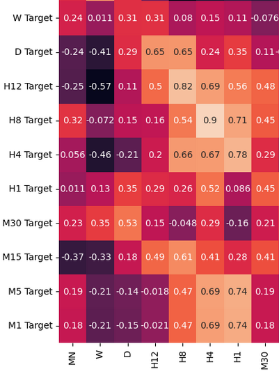
Fig 3: A few of values from the correlation matrix we obtained

Performing a scatter-plot of the monthly and weekly close prices had an unclear trend in it. For the most part, it appears the data has a general uptrend to it.

sns.scatterplot(data=prices,x="MN Close",y="W Close")

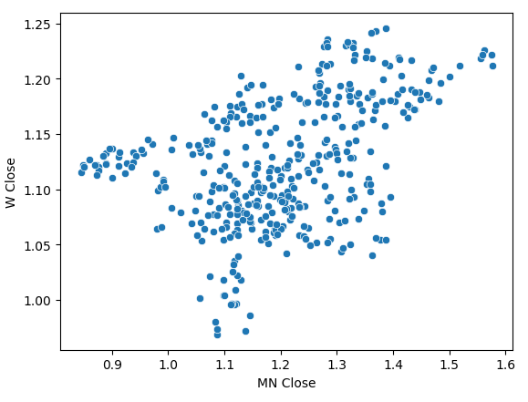
Fig 4: A scatter plot of our monthly and weekly close prices

We transformed our price data to periodic returns and performed the scatter plot again. This time a general trend appears, it appears our returns cluster around 0.

sns.scatterplot(data=prices.pct_change(),x="MN Close",y="W Close")

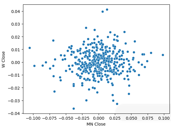
Fig 5: A scatter plot of our returns on different time-frames

When we performed box plots of our returns over different time-frames, we can observe another trend. The variance in our returns decreases as we move away from the monthly time-frame, down to lower time-frames. Likewise, the average return across all time frames is close to 0. This can also be interpreted to tell us that if we are trying to maximize the returns on a portfolio, we should consider higher time-frames.

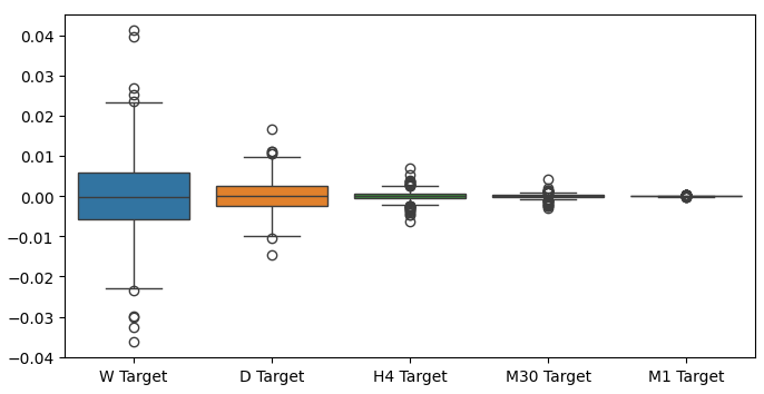
Fig 6: A box-plot of our returns across different time-frames

Preparing To Model The Data

Let us now make the preparations needed to begin modelling the data. First, we need to make train-test splits of our data.

#Create train test splits
X_train_mn,X_test_mn,y_train_mn,y_test_mn      = train_test_split(prices.loc[:,["MN"]],prices.loc[:,"MN Target"],test_size=0.5,shuffle=False)
X_train_w,X_test_w,y_train_w,y_test_w          = train_test_split(prices.loc[:,["W"]],prices.loc[:,"W Target"],test_size=0.5,shuffle=False)
X_train_d,X_test_d,y_train_d,y_test_d          = train_test_split(prices.loc[:,["D"]],prices.loc[:,"D Target"],test_size=0.5,shuffle=False)
X_train_h12,X_test_h12,y_train_h12,y_test_h12  = train_test_split(prices.loc[:,["H12"]],prices.loc[:,"H12 Target"],test_size=0.5,shuffle=False)
X_train_h8,X_test_h8,y_train_h8,y_test_h8      = train_test_split(prices.loc[:,["H8"]],prices.loc[:,"H8 Target"],test_size=0.5,shuffle=False)
X_train_h4,X_test_h4,y_train_h4,y_test_h4      = train_test_split(prices.loc[:,["H4"]],prices.loc[:,"H4 Target"],test_size=0.5,shuffle=False)
X_train_h1,X_test_h1,y_train_h1,y_test_h1      = train_test_split(prices.loc[:,["H1"]],prices.loc[:,"H1 Target"],test_size=0.5,shuffle=False)
X_train_m30,X_test_m30,y_train_m30,y_test_m30  = train_test_split(prices.loc[:,["M30"]],prices.loc[:,"M30 Target"],test_size=0.5,shuffle=False)
X_train_m15,X_test_m15,y_train_m15,y_test_m15  = train_test_split(prices.loc[:,["M15"]],prices.loc[:,"M15 Target"],test_size=0.5,shuffle=False)
X_train_m5,X_test_m5,y_train_m5,y_test_m5      = train_test_split(prices.loc[:,["M5"]],prices.loc[:,"M5 Target"],test_size=0.5,shuffle=False)
X_train_m1,X_test_m1,y_train_m1,y_test_m1      = train_test_split(prices.loc[:,["M1"]],prices.loc[:,"M1 Target"],test_size=0.5,shuffle=False)

Now store these splits into lists.

train_X = [
X_train_mn,
X_train_w,
X_train_d,
X_train_h12,
X_train_h8,
X_train_h4,
X_train_h1,
X_train_m30,
X_train_m15,
X_train_m5,
X_train_m1
]

test_X = [
X_test_mn,
X_test_w,
X_test_d,
X_test_h12,
X_test_h8,
X_test_h4,
X_test_h1,
X_test_m30,
X_test_m15,
X_test_m5,
X_test_m1
]

Repeat the above procedure for the target values.

train_y = [
y_train_mn,
y_train_w,
y_train_d,
y_train_h12,
y_train_h8,
y_train_h4,
y_train_h1,
y_train_m30,
y_train_m15,
y_train_m5,
y_train_m1,
]

test_y = [
y_test_mn,
y_test_w,
y_test_d,
y_test_h12,
y_test_h8,
y_test_h4,
y_test_h1,
y_test_m30,
y_test_m15,
y_test_m5,
y_test_m1,
]

Cross-validate each model.

#Record our error 
for i in np.arange(0,len(train_X)):
    #Fit the model
    model = LinearRegression()
    cv_score = cross_val_score(model,train_X[i],train_y[i],cv=5)
    error_levels.iloc[0,i] = np.mean(cv_score * -1)
    #Record validation error
    model.fit(train_X[i],train_y[i])
    test_error_levels.iloc[0,i] = mean_squared_error(test_y[i],model.predict(test_X[i]))

Our respective error levels.

error_levels

MN	W	D	H12	H8	H4	H1	M30	M15	M5	M1
0.719131	3.979435	3.897228	5.023601	5.218168	40.406227	0.196244	18.264356	3.680168	20.331821	3.540946

Let us visualize our approximation of the distribution of our model's residual.

fig, ax = plt.subplots(figsize=(7,4)) 
sns.barplot(error_levels,ax=ax)

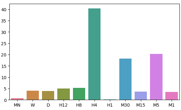
Fig 7: Visualizing our model's error levels

Feature Importance

Now that we have identified our optimal time-frames, let us try and detect if there may be any causality at play between the 2 time-frames. In 1969, Sir Clive Granger proposed a test to empirically determine if two time-series data caused each other, even in cases where past values of 1 time-series, affected future values of the latter. Put simply, Granger's test is passed if we can lag the values of one time-series and use it to predict the future value of the second without a significant drop in variance of our predictions.

Since its inception, the Granger test has undergone many changes and improvements. In modern times, it is widely used across industries from neuroscience to finance. The use of the test has been at the center of much debate in academic circles for over half a century now. The bulk of the problem lies in the assumptions of linearity that are implicitly made by Granger's test. Therefore, if there is true a causal relationship that is non-linear, Granger's test will refute its existence. Furthermore, in practice, the test is typically constrained to bi-variate problems. That is to say, we rarely ever use Granger's test on large problems with more than 2 time-series datasets.

Fig 8: The Late British Economist Sir Clive Granger

To get started, let us first import the statsmodels library and then run the test. The test is performed over lagged versions of the H1 Close. The test is passed if we obtain p-values < 0.05, which we did on the first lag. All subsequent lags failed the test and we can reject there is any causality beyond the first lag.

from statsmodels.tsa.stattools import grangercausalitytests

result = grangercausalitytests(prices[['H1 Close','MN Close']].pct_change().dropna(), maxlag=4)

Granger Causality
number of lags (no zero) 1
ssr based F test:         F=4.4913 , p=0.0347 , df_denom=395, df_num=1
ssr based chi2 test:   chi2=4.5254 , p=0.0334 , df=1
likelihood ratio test: chi2=4.4999 , p=0.0339 , df=1
parameter F test:         F=4.4913 , p=0.0347 , df_denom=395, df_num=1

Granger Causality
number of lags (no zero) 2
ssr based F test:         F=2.2706 , p=0.1046 , df_denom=392, df_num=2
ssr based chi2 test:   chi2=4.5991 , p=0.1003 , df=2
likelihood ratio test: chi2=4.5727 , p=0.1016 , df=2
parameter F test:         F=2.2706 , p=0.1046 , df_denom=392, df_num=2

Granger's causality normally works one way. Let us ensure this by checking for causality in the opposite direction. None of the p-values obtained were significant, reassuring us that the causality is indeed going one way as we expect.

result = grangercausalitytests(prices[['MN Close','H1 Close']].pct_change().dropna(), maxlag=4)

Granger Causality
number of lags (no zero) 1
ssr based F test:         F=0.0188 , p=0.8909 , df_denom=395, df_num=1
ssr based chi2 test:   chi2=0.0190 , p=0.8905 , df=1
likelihood ratio test: chi2=0.0190 , p=0.8905 , df=1
parameter F test:         F=0.0188 , p=0.8909 , df_denom=395, df_num=1

Granger Causality
number of lags (no zero) 2
ssr based F test:         F=2.2182 , p=0.1102 , df_denom=392, df_num=2
ssr based chi2 test:   chi2=4.4930 , p=0.1058 , df=2
likelihood ratio test: chi2=4.4678 , p=0.1071 , df=2
parameter F test:         F=2.2182 , p=0.1102 , df_denom=392, df_num=2

Granger Causality
number of lags (no zero) 3
ssr based F test:         F=1.7310 , p=0.1601 , df_denom=389, df_num=3
ssr based chi2 test:   chi2=5.2863 , p=0.1520 , df=3
likelihood ratio test: chi2=5.2513 , p=0.1543 , df=3
parameter F test:         F=1.7310 , p=0.1601 , df_denom=389, df_num=3

Granger Causality
number of lags (no zero) 4
ssr based F test:         F=1.4694 , p=0.2108 , df_denom=386, df_num=4
ssr based chi2 test:   chi2=6.0148 , p=0.1980 , df=4
likelihood ratio test: chi2=5.9694 , p=0.2014 , df=4
parameter F test:         F=1.4694 , p=0.2108 , df_denom=386, df_num=4

Dynamic Time Series Warping also allows us to find similarities between two time-series data-sets. The algorithm can also be used to align series of different lengths. We employed the algorithm to find points of similarity between the monthly and hourly returns of our data. The algorithm accomplishes this task by minimizing a specialized cost function that measures the difference between 2 series. We will start by importing the libraries we need.

#Let's calculate the simillarities between our time series data
from dtaidistance import dtw
from dtaidistance import dtw_visualisation as dtwvis

Now let us find similarities between the returns.

series_1 = prices["MN Close"].pct_change(periods=1).dropna().reset_index(drop=True) * 100
series_2 = prices["H1 Close"].pct_change(periods=1).dropna().reset_index(drop=True) * 100
path = dtw.warping_path(series_1, series_2)
dtwvis.plot_warping(series_1, series_2, path)

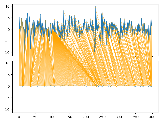
Fig 9: Visualizing the similarities between the monthly and hourly returns

Parameter Tuning

Let us now tune the parameters of our Deep Neural Network to outperform the benchmark performance set by our Linear Regression. Note that due to the nature of the optimization procedures used to train DNN, the results obtained in this section of the article may be challenging to reproduce. As a matter of fact, I ran this test 5 times, and we failed to our perform the Linear model on 2 tests.

Import the libraries we need, and initialize the model.

#Let's try to outperform our linear regression model
from sklearn.neural_network import MLPRegressor
from sklearn.model_selection import RandomizedSearchCV

#Let's tune our model
model = MLPRegressor(max_iter=500)

Define the parameter space.

#Tuner 
tuner = RandomizedSearchCV(
    model,
        {
        "activation" : ["relu","logistic","tanh","identity"],
        "solver":["adam","sgd","lbfgs"],
        "alpha":[0.1,0.01,0.001,0.0001,0.00001,0.00001,0.0000001,0.000000001,0.000000000000001],
        "tol":[0.1,0.01,0.001,0.0001,0.00001,0.000001,0.0000001,0.000000001,0.000000000000001],
        "learning_rate":['constant','adaptive','invscaling'],
        "learning_rate_init":[1,0.1,0.0001,0.000001,100,10000,1000000,1000000000,100,1000],
        "shuffle": [True,False],
        "hidden_layer_sizes":[(1,4),(1,4,5),(1,8,10),(2,5),(8),(10,12),(5,10,4)]
        },
        n_iter=100,
        cv=5,
        n_jobs=-1,
        scoring="neg_mean_squared_error"
)

Fit the tuner.

tuner.fit(X_train_mn,y_train_mn)

The best parameters we found.

tuner.best_params_

{'tol': 0.001,
'solver': 'lbfgs',
'shuffle': True,
'learning_rate_init': 1,
'learning_rate': 'adaptive',
'hidden_layer_sizes': (2, 5),
'alpha': 1e-05,
'activation': 'identity'}

Deeper Optimization

Let us perform a deeper search for optimal parameters using the SciPy library.

#Deeper optimization
from scipy.optimize import minimize

Create data structures to record our progress.

#Create a dataframe to store our accuracy
current_error_rate = pd.DataFrame(index = np.arange(0,5),columns=["Current Error"])
optimization_progress = []

Define the objective function to be minimized. We want to minimize our model's root mean squared error.

#Define the objective function
def objective(x):
    #The parameter x represents a new value for our neural network's settings
    #In order to find optimal settings, we will perform 10 fold cross validation using the new setting
    #And return the average RMSE from all 10 tests
    #We will first turn the model's Alpha parameter, which controls the amount of L2 regularization
    model = MLPRegressor(hidden_layer_sizes=tuner.best_params_["hidden_layer_sizes"],
                         activation=tuner.best_params_["activation"],
                         learning_rate=tuner.best_params_["learning_rate"],
                         solver=tuner.best_params_["solver"],
                         shuffle=tuner.best_params_["shuffle"],
                         alpha=x[0],
                         tol=x[1],
                         learning_rate_init=x[2])
    #Now we will cross validate the model
    for i,(train,test) in enumerate(tscv.split(X_train_mn)):
        #Train the model
        model.fit(X_train_mn.loc[train[0]:train[-1],:],y_train_mn.loc[train[0]:train[-1]])
        #Measure the RMSE
        current_error_rate.iloc[i,0] = mean_squared_error(y_train_mn.loc[test[0]:test[-1]],model.predict(X_train_mn.loc[test[0]:test[-1],:]))
    #Record the progress made by the optimizer
    optimization_progress.append(current_error_rate.iloc[:,0].mean())
    #Return the Mean CV RMSE
    return(current_error_rate.iloc[:,0].mean())

Specify the starting point for the optimization procedure and specify large bounds so that we can approximate global optimization.

#Define the starting point
pt = [tuner.best_params_["alpha"],tuner.best_params_["tol"],tuner.best_params_["learning_rate_init"]]
bnds = ((0.000000001,10000000000),(0.0000000001,10000000000),(0.000000001,10000000000))

Optimizing our DNN model.

#Searchin deeper for parameters
result = minimize(objective,pt,method="TNC",bounds=bnds)

It appears we performed the optimization successfully.

result

message: Converged (|x_n-x_(n-1)| ~= 0)
success: True
status: 2
     fun: 0.04257403904271943
       x: [ 4.864e-05 1.122e-03 9.999e-01]
     nit: 1
     jac: [ 1.298e+04 1.806e+02 -3.371e+03]
    nfev: 92

Store our optimal values.

optima_y = result.fun
optima_x = optimization_progress.index(optima_y)
inputs = np.arange(0,len(optimization_progress))

Visualize the progress made by the Optimization procedure.

plt.scatter(inputs,optimization_progress)
plt.plot(optima_x,optima_y,'s',color='r')
plt.axvline(x=optima_x,ls='--',color='red')
plt.axhline(y=optima_y,ls='--',color='red')
plt.title("Minimizing Training MSE")

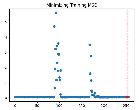
Fig 10: The results of our TNC optimization procedure

Testing For Overfitting

Let us see if we can indeed outperform our default linear model.

#Test for overfitting
benchmark = LinearRegression()

default_model = MLPRegressor(max_iter=200)

random_search_model = MLPRegressor(hidden_layer_sizes=tuner.best_params_["hidden_layer_sizes"],
                         activation=tuner.best_params_["activation"],
                         learning_rate=tuner.best_params_["learning_rate"],
                         solver=tuner.best_params_["solver"],
                         shuffle=tuner.best_params_["shuffle"],
                         alpha=tuner.best_params_["alpha"],
                         tol=tuner.best_params_["tol"],
                         learning_rate_init=tuner.best_params_["learning_rate_init"],
                         max_iter=200
                        )

lbfgs_model = MLPRegressor(hidden_layer_sizes=tuner.best_params_["hidden_layer_sizes"],
                         activation=tuner.best_params_["activation"],
                         learning_rate=tuner.best_params_["learning_rate"],
                         solver=tuner.best_params_["solver"],
                         shuffle=tuner.best_params_["shuffle"],
                         alpha=result.x[0],
                         tol=result.x[1],
                         learning_rate_init=result.x[2],
                         max_iter=200
                        )

Fit the models on the training set.

#Fit the models
benchmark.fit(X_train_mn,y_train_mn)
default_model.fit(X_train_mn,y_train_mn)
random_search_model.fit(X_train_mn,y_train_mn)
lbfgs_model.fit(X_train_mn,y_train_mn)

Make preparations to record our cross-validation scores.

#Record our cross val scores
models = [benchmark,
          default_model,
          random_search_model,
          lbfgs_model
         ]

val_error = pd.DataFrame(columns=["Linear Reg","Default NN","Random Search NN","TNC NN"],index=[0])

Cross-validate each model.

for i in np.arange(0,len(models)):
    val_error.iloc[0,i] = np.mean(cross_val_score(models[i],X_test_mn,y_test_mn,cv=5,n_jobs=-1)) * -1

Our validation error clearly shows our TNC optimized neural network was the best performing.

val_error

Linear Reg	Default NN	Random Search NN	TNC NN
3.323741	3.987083	3.314776	3.283775

Exporting To ONNX Format

Let us now prepare to export our model to ONNX format. ONNX stands for Open Neural Network Exchange, and it is an open-source protocol for representing any machine learning model as a tree of nodes representing calculations and the flow of data after each calculation. ONNX allows us to build and use machine learning models in different programming languages, provided those languages implement the ONNX specification.

Import the ONNX library to get started.

#Preparing to export to ONNX
import onnx
from skl2onnx import convert_sklearn
from skl2onnx.common.data_types import FloatTensorType

Prepare the model.

#Fit the model on all the data we have 
model = MLPRegressor(
 solver= 'lbfgs',
 shuffle= True,
 activation= 'identity',
 learning_rate= 'adaptive',
 hidden_layer_sizes= (2, 5),
 alpha= 4.864e-05,
 tol= 1.122e-03,
 learning_rate_init= 9.999e-01,
)

Fit the model on all the data we have.

model.fit(prices[["MN Close"]],prices.loc[:,"MN Target"])

Define the input shape of our model.

#Define the input types for our ONNX model
initial_types = [("float_input",FloatTensorType([1,1]))]

Create the ONNX representation of the model.

# Create the ONNX representation
onnx_model = convert_sklearn(model,initial_types=initial_types,target_opset=12)

Export the model to ONNX format.

# Save the ONNX model
onnx.save_model(onnx_model,"EURUSD MN1 AI.onnx")

Let us now visualize our model in ONNX format to ensure our inputs are the right size.

import netron

netron.start("EURUSD MN1 AI.onnx")

Visualizing our DNN

Fig 11: Visualizing our DNN model

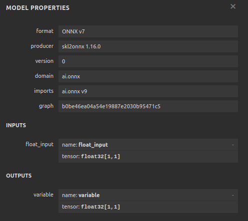
Fig 12: Our model's I/O shape

Implementing in MQL5

We want to now implement our trading algorithm in MQL5. We desire our trading algorithm to be able to switch between closing its positions using simple moving averages and using AI predictions. Furthermore, we want to guide our AI model using technical analysis. To get started, we will first import the ONNX model we exported above.

//+------------------------------------------------------------------+
//|                                                EURUSD MTF AI.mq5 |
//|                                        Gamuchirai Zororo Ndawana |
//|                          https://www.mql5.com/en/gamuchiraindawa |
//+------------------------------------------------------------------+
#property copyright "Gamuchirai Zororo Ndawana"
#property link      "https://www.mql5.com/en/gamuchiraindawa"
#property version   "1.00"

//+------------------------------------------------------------------+
//| Load the ONNX resources                                          |
//+------------------------------------------------------------------+
#resource "\\Files\\EURUSD MN1 AI.onnx" as const uchar onnx_buffer[];

Now we will define our custom enumerator to specify how the user would like to close positions.

//+-------------------------------------------------------------------+
//| Define our custom type                                            |
//+-------------------------------------------------------------------+
enum close_type
  {
   MA_CLOSE = 0, // Moving Averages Close
   AI_CLOSE = 1  // AI Auto Close
  };

Let us create inputs, so we can change how our application closes its positions to see which is better.

//+------------------------------------------------------------------+
//| User inputs                                                      |
//+------------------------------------------------------------------+
input close_type user_close_type = AI_CLOSE; // How should we close our positions?

We need to import the trade class.

//+------------------------------------------------------------------+
//| Libraries we need                                                |
//+------------------------------------------------------------------+
#include <Trade\Trade.mqh>
CTrade Trade;

Create global variables we will need throughout our program.

//+------------------------------------------------------------------+
//| Global variables                                                 |
//+------------------------------------------------------------------+
long    onnx_model;
vectorf model_input  = vectorf::Zeros(1);
vectorf model_output = vectorf::Zeros(1);
double  bid,ask;
int     ma_hanlder;
double  ma_buffer[];
int     bb_hanlder;
double  bb_mid_buffer[];
double  bb_high_buffer[];
double  bb_low_buffer[];
int     rsi_hanlder;
double  rsi_buffer[];
int     system_state = 0,model_state=0;

When our application is being loaded, we will first create our ONNX model from the buffer we created earlier. Then we will assign our technical indicator handlers.

//+------------------------------------------------------------------+
//| Expert initialization function                                   |
//+------------------------------------------------------------------+
int OnInit()
  {
//--- Load our ONNX function
   if(!load_onnx_model())
     {
      return(INIT_FAILED);
     }

//--- Load our technical indicators
   bb_hanlder  = iBands("EURUSD",PERIOD_D1,30,0,1,PRICE_CLOSE);
   rsi_hanlder = iRSI("EURUSD",PERIOD_D1,14,PRICE_CLOSE);
   ma_hanlder  = iMA("EURUSD",PERIOD_D1,20,0,MODE_EMA,PRICE_CLOSE);

//---
   return(INIT_SUCCEEDED);
  }

If our Expert Advisor is removed off the chart, we should release the resources we are no longer using.

//+------------------------------------------------------------------+
//| Expert deinitialization function                                 |
//+------------------------------------------------------------------+
void OnDeinit(const int reason)
  {
//--- Release the resources we don't need
   release_resources();
  }

Now, whenever we receive updated prices, we will first store the new technical data, make a prediction from our model and then display important stats back to the user. If we have no open positions, we will follow our model's predictions. Otherwise, we will follow the user's inputs to determine if we should keep our positions open or closed.

//+------------------------------------------------------------------+
//| Expert tick function                                             |
//+------------------------------------------------------------------+
void OnTick()
  {
//--- Update market data
   update_market_data();

//--- Fetch a prediction from our model
   model_predict();

//--- Display stats
   display_stats();

//--- Find a position
   if(PositionsTotal() == 0)
     {
      if(model_state == 1)
         check_bullish_setup();
      else
         if(model_state == -1)
            check_bearish_setup();
     }

//--- Manage the position we have
   else
     {
      //--- How should we close our positions?
      if(user_close_type == MA_CLOSE)
        {
         ma_close_positions();
        }

      else
        {
         ai_close_positions();
        }

     }
  }
//+------------------------------------------------------------------+

Let us now define how our AI system should close its trades. If our AI system is detecting price levels will change in a manner that contradicts our position's assertion, we will close our trades.

//+------------------------------------------------------------------+
//| Close whenever our AI detects a reversal                         |
//+------------------------------------------------------------------+
void ai_close_positions(void)
  {
   if(system_state != model_state)
     {
      Alert("Reversal detected by our AI system,closing open positions");
      Trade.PositionClose("EURUSD");
     }
  }

On the other hand, if we shall rely on the moving average to close our positions, then we want to close any sell trades if the closing price is above the moving average and vice versa for our sell trades.

//+------------------------------------------------------------------+
//| Close whenever price reverses the moving average                 |
//+------------------------------------------------------------------+
void ma_close_positions(void)
  {
//--- Is our buy position possibly weakening?
   if(system_state == 1)
     {
      if(iClose("EURUSD",PERIOD_D1,0) < ma_buffer[0])
         Trade.PositionClose("EURUSD");
     }
//--- Is our sell position possibly weakening?
   if(system_state == -1)
     {
      if(iClose("EURUSD",PERIOD_D1,0) > ma_buffer[0])
         Trade.PositionClose("EURUSD");
     }
  }

For us to open a trade, we will firs require a Bollinger Band breakout followed with confirmation from the RSI indicator, and lastly we would also want to see the moving average on the right side in relation to price.

//+------------------------------------------------------------------+
//| Check bearish setup                                              |
//+------------------------------------------------------------------+
void check_bearish_setup(void)
  {
   if(iClose("EURUSD",PERIOD_D1,0) < bb_low_buffer[0])
     {
      if(50 > rsi_buffer[0])
        {
         if(iClose("EURUSD",PERIOD_D1,0) < ma_buffer[0])
           {
            Trade.Sell(0.3,"EURUSD",bid,0,0,"EURUSD MTF AI");
            system_state = -1;
           }
        }
     }
  }

//+------------------------------------------------------------------+
//| Check bullish setup                                              |
//+------------------------------------------------------------------+
void check_bullish_setup(void)
  {
   if(iClose("EURUSD",PERIOD_D1,0) > bb_high_buffer[0])
     {
      if(50 < rsi_buffer[0])
        {
         if(iClose("EURUSD",PERIOD_D1,0) > ma_buffer[0])
           {
            Trade.Buy(0.3,"EURUSD",ask,0,0,"EURUSD MTF AI");
            system_state = 1;
           }
        }
     }
  }

This function will currently display just the model's prediction.

//+------------------------------------------------------------------+
//| Display account stats                                            |
//+------------------------------------------------------------------+
void display_stats(void)
  {
   Comment("Forecast: ",model_output[0]);
  }

Fetching a prediction from our model and storing it using a binary flag.

//+------------------------------------------------------------------+
//| Fetch a prediction from our model                                |
//+------------------------------------------------------------------+
void model_predict(void)
  {
//--- Get inputs
   model_input.CopyRates("EURUSD",PERIOD_MN1,COPY_RATES_CLOSE,0,1);
//--- Fetch a prediction from our model
   OnnxRun(onnx_model,ONNX_DEFAULT,model_input,model_output);
//--- Store the model's prediction as a flag
   if(model_output[0] > model_input[0])
     {
      model_state = -1;
     }
   else
      if(model_output[0] < model_input[0])
        {
         model_state = 1;
        }
  }

Let us now specify the function that will release the resources we do not need.

//+------------------------------------------------------------------+
//| Release the resources we don't need                              |
//+------------------------------------------------------------------+
void release_resources(void)
  {
   OnnxRelease(onnx_model);
   IndicatorRelease(ma_hanlder);
   IndicatorRelease(rsi_hanlder);
   IndicatorRelease(bb_hanlder);
   ExpertRemove();
  }

Whenever a new price is quoted, this function will be called to update the market data we have.

//+------------------------------------------------------------------+
//| Update our market data                                           |
//+------------------------------------------------------------------+
void update_market_data(void)
  {
//--- Update all our technical data
   bid = SymbolInfoDouble("EURUSD",SYMBOL_BID);
   ask = SymbolInfoDouble("EURUSD",SYMBOL_ASK);
   CopyBuffer(ma_hanlder,0,0,1,ma_buffer);
   CopyBuffer(rsi_hanlder,0,0,1,rsi_buffer);
   CopyBuffer(bb_hanlder,0,0,1,bb_mid_buffer);
   CopyBuffer(bb_hanlder,1,0,1,bb_high_buffer);
   CopyBuffer(bb_hanlder,2,0,1,bb_low_buffer);
  }

Lastly, let us define the function that will create our ONNX model from the buffer we defined earlier.

//+------------------------------------------------------------------+
//| Load our ONNX model                                              |
//+------------------------------------------------------------------+
bool load_onnx_model(void)
  {
//--- Create the ONNX model from our buffer
   onnx_model = OnnxCreateFromBuffer(onnx_buffer,ONNX_DEFAULT);

//--- Validate the model
   if(onnx_model == INVALID_HANDLE)
     {
      //--- Give feedback
      Comment("Failed to create the ONNX model");
      //--- We failed to create the model
      return(false);
     }

//--- Specify the I/O shapes
   ulong input_shape[] = {1,1};
   ulong output_shape[] = {1,1};

//--- Validate the I/O shapes
   if(!(OnnxSetInputShape(onnx_model,0,input_shape)) || !(OnnxSetOutputShape(onnx_model,0,output_shape)))
     {
      //--- Give feedback
      Comment("We failed to define the correct input shapes");

      //--- We failed to define the correct I/O shape
      return(false);
     }

   return(true);
  }
//+------------------------------------------------------------------+

Our Expert Advisor in Action

Fig 13: Our Expert Advisor's inputs

Our system in action

Fig 14: Our Expert Advisor in action

Our backtest history

Fig 15: The results of back-testing our strategy

Backtesting our strategy

Fig 16: Our strategy's walk forward testing results

Conclusion

In this article, we have demonstrated that the monthly and hourly time-frames appear to be the most stable for predicting the EURUSD pair. We cannot be confident that this holds true for every existing market. Likewise, we must also in future consider searching more possible time-frames to ensure that we are not overlooking any optimal time-frames. Additionally, there are further adjustments we can make to our approach to search for lower error metrics. For example, we may be curious to understand whether there is a combination of timeframes that could lower our error levels even further.

Attached files |

Download ZIP

EURUSD_MTF_AI.mq5 (9.23 KB)

Multiple_Time_Frame_Analysis.ipynb (1243.36 KB)

EURUSD_MN1_AI.onnx (0.83 KB)

Warning: All rights to these materials are reserved by MetaQuotes Ltd. Copying or reprinting of these materials in whole or in part is prohibited.