MQL5 Wizard Techniques you should know (Part 57): Supervised Learning with Moving Average and Stochastic Oscillator

Introduction

We continue our look at simple patterns that can be implemented with MQL wizard assembled Expert Advisors. The primary purpose of this is always to pilot or test drive ideas. Eventual deployment and live account use can use manually assembled Expert Advisors after testing over longer periods, but wizard assembled Experts allow quick test runs with less upfront code.

Machine Learning is all the rage at the moment, and we have covered some specific aspects of it in previous articles of these series. We will continue to cover some of these more technical features in this and future articles, however they will be a backdrop since we will be more focused on better known and established indicator patterns.

Furthermore, in the context of machine learning, our articles will cover the 3 main branches of learning in separate articles each, in a cycle. To start off we will look at supervision or supervised-learning and our indicator patterns will be from the pairing of a trend indicator and a momentum indicator. We will be looking at the Moving Average and Stochastic Indicators.

In supervised learning, we will seek to implement each pattern in a separate neural network. These, as argued in recent articles, are better coded and trained in python than MQL5. The efficiency gains are off the charts. Python also easily allows testing for cross validation following a training session, and thus we will be performing these for each pattern.

While cross validation is shared in Python by comparing loss value of test run to loss value of last training epoch, this alone, though important, is bound to be insufficient in assessing the cross validation of the network's current weights and biases. 

We will therefore be performing forward walk runs in the MetaTrader 5 strategy tester, with the exported ONNX networks. For this piece, the pricing or x and y datasets that are sent to python from MetaTrader 5 to begin the training will be for the year 2023, for the pair EUR JPY. Therefore, the forward walk will be for the same symbol but the year 2024. We are performing our analysis on the Daily time frame.

Combining the Moving Average (MA) with the Stochastic Oscillator can generate a variety of trading signals. For our testing and exploring purposes, we will only consider the 10 top signal patterns that traders can use when these indicators are combined.

Approach with Machine Learning Types

A machine learning pipeline can be viewed as these 3 interconnected phases; Supervision, Reinforcement, & Inference. Let's recap on the definitions of each.

Supervised-Learning (aka the Training Phase) – is when the model learns historical patterns based on labelled data (independent or input data often labelled x, and independent data to forecast also often labelled y). 

Meanwhile,  Reinforcement-Learning (which can be seen as in-use Learning & Optimization phase) – can be taken as a stage where the model refines itself through interaction with its environment, and optimization of its actions for long-term rewards (almost like backpropagation during a forward walk). And finally 

And finally, Inference-Learning (akaUnsupervised-Learning phase) – would be when the model is generalizing from past learning and applying what was learnt to new data and new problems.

Purely for illustration, let's look at how these 3 phases could be linked when dealing with different sets of problems. We will consider cases of weather information systems and financial time series forecasting.

Supervision:

Supervised learning's Goal is to generate a predictive model from labelled data. This process involves collecting and pre-processing of Historical data. This is then followed by feature extraction, which could be taken as a form of normalizing the historic data to a range or format that can be inputted into the neural network or training model. After this the model gets trained on LSTMs, or XGBoost or transformers using labelled data. Labelling means we mark the independent data (precursor data that is known and is used to forecast) and dependent data (the data we want to predict) with distinct labels. The initial goal here is loss minimization, having the difference between predicted and actual as small as possible by using gradient descent.

In supervised learning, cross validation can be involved, and its results can make the case for deploying the model to full use. However, with the 3 pronged steps that we're exploring here, the final stage of supervised learning would be model Selection & hyperparameter tuning where in essence the optimal learning rate and training batch size are chosen based on what worked best. Also, the architecture with regard to activation types, and even layer sizes is chosen if these options were tested in this training phase.

To illustrate this, in a weather forecasting system: the data would be past temperature, humidity, or pressure; the model could be a random forest or CNN-based model; with the outcome being a system for predicting temperature trends.  With financial time series, forecasting data would be Historical prices with feature Engineering to give indicator values; the model could be LSTM; loss function MSE; and the outcome being a trained model that predicts the next price based on past observations.

Reinforcement:

Having performed supervised learning which is largely on labelled historical data, the question then becomes will the model be able to perform on live or future data? Or will it even be able to adapt should future conditions change from what it trained on? To answer this Reinforcement, learning is engaged. Static models usually struggle in dynamic environments, which is why Reinforcement Learning helps optimize the decision-making process going forward.

The goal of RL therefore is to improve forecasts by optimizing decision-making based on feedback. Put differently, once we have, say , a neural network that forecasts changes in price, we would then proceed to develop policy and value network(s) that are able to use these price changes as states. We are thus in a position where we separate price changes from trader actions, with the introduction of states and actions.

These examples are for financial time series forecasting , if it was weather as we illustrated above then the states’ and actions could be the amount of rainfall, and how much to sow/ plant a major crop. A more tangible and desired result of the financial time series forecasting is often profits/ losses from actions taken in following the network's forecasts. For our weather illustration, this could be the yields from the major crop.

The RL process as we covered previously not only involves training and updating the critic-network so we can better anticipate our profits/ loss position, but it also provides deltas that further fine tune the weights and biases of the policy network.

The RL process, to recap, involves: Agent-Environment setup where states, actions and rewards get defined. As mentioned these would be flowing or determined from the model trained at the supervision phase (as shown with illustrations above); Then also policy-learning where an actor network or equivalent algorithm is optimized to map states to their required actions; Also a Reward based optimization mechanism which can take the form of a value-algorithm or critic-network that adjusts predictions based on long-term profitability; And finally an agent that balances exploration (the trying out of different policy settings with the goal of learning something new) against exploitation (sticking to what has worked well in the past).

If we can use examples to show what happens here with  weather and financial forecasting as above in the supervision phase; with the weather prediction at the supervision phase the initial model predicts rainfall based on temperature, humidity etc and outputs of projected rainfall that we seek. Because this rainfall is a key determinant on whether we should do planting for our crop, RL introduces a decision layer of interpretation. The rain forecast output becomes cast as states. If these states forecast different precipitation in different regions or points in time, their interpretation in determining whether to plant can be optimized towards a reward, which in this case would be the crop yield. The outcome of this would be a forecasting model that improves itself in response to real-world weather shifts. So, if the supervision phase was school, then reinforcement is on job training.

For financial forecasting, we would have forecast price changes from the model at the supervision stage, acting as our state. These changes can still be a multidimensional vector if for instance they encompass more than one time frame. The actions would be those taken by the trader or Expert Advisor which are to either buy, sell, or be neutral. Based on the actions taken for each state (price changes) we would then map by critic-network or algorithm, the states and actions to the expected profits, for each. Once this is done, the policy (mapping of states to actions) can be updated gradually by balancing exploration with exploitation to better interpret the outputs of the model in the supervision stage (which outputs we cast as states).

This on-job training, though, means that it happens very slowly by default because live data only trickles out at a very tepid pace. So if you supervised-training covered a historical period of 10 years, reinforcement training for a period of 1 year, would on paper also take 1 year! This therefore necessitates the need for simulation or a more elaborate environment class.

By simulating live data conditions on a set of historical data, we do not just quicken the pace of reinforcement learning, but we also cover a lot more data which should provide us with more resilient models. 

So, for the financial series forecasting, this means we can make test runs on the same data we used in supervision but now optimize the RL networks for profit by basing this on the actions taken given the state (or price change) forecasts made with the network at the supervision stage. 

Inference:

Having got 2 models, one for making the basis forecasts (in supervised learning) and one for better interpreting and applying these forecasts (in reinforcement) we are then presented with the 3rd phase, inference, where in essence we take this knowledge and models and apply it to a different field or as the case may be in our situation a different trade symbol.

This is also referred to as generalizing on unseen data. The application of learned knowledge in real-world settings, refining it over time, and detecting unseen patterns without using labels on the data. Graphs and auto-encoders play very key roles in this phase, as well as clustering. 

In these 3 phases, with each progression to the next, the compute overloads get diminished. Which again, in essence, is the justification for these phases. Methods that engage unsupervised learning have been looked at so far in these series, however I may revisit them soon with an eye on how they can “carry-on” from reinforcement learning. Even though RL can be used autonomously in forecasting these outlined phases seek to make the case it may be more efficient to use it with the other modes of learning.

Combining the Moving Average (MA) with the Stochastic Oscillator can generate a variety of trading signals. We examine the top 10 signal patterns that are generated from combining these indicators that traders could use.

Moving Average Crossover + Stochastic Overbought/Oversold

This pattern coming from the combination of a trend following indicator (MA), and momentum oscillator (the stochastic) does tend to provide high probability setups. The buy Signal is a bullish crossover (where the quick MA crosses above the Lagging MA) to confirm a potential uptrend, all the while the Stochastic Oscillator is below 20. This usually suggests the asset is oversold, and the price is ready for reversal. The sell Signal on the flip side is a bearish crossover. This indicates the quick MA crossing the Lagging MA from above to go below it, which by itself is potentially a downtrend indicator. Since this is also supposed to be backed by the Stochastic being above the 80 level, a sign of overbought conditions, it does form a strong-sell Signal. 

With our slightly modified signal class format where we use indicator readings as features for networks, we now have a solo pattern function that we code as follows:

//+------------------------------------------------------------------+
//| Check for Pattern.                                               |
//+------------------------------------------------------------------+
double CSignal_MA_STO::IsPattern(int Index, ENUM_POSITION_TYPE T)
{  vectorf _x = Get(Index, m_time.GetData(X()), m_close, m_ma, m_ma_lag, m_sto);
   vectorf _y(1);
   _y.Fill(0.0);
   ResetLastError();
   if(!OnnxRun(m_handles[Index], ONNX_NO_CONVERSION, _x, _y))
   {  printf(__FUNCSIG__ + " failed to get y forecast, err: %i", GetLastError());
      return(double(_y[0]));
   }
   //printf(__FUNCSIG__+" y: "+DoubleToString(_y[0],2));
   if(T == POSITION_TYPE_BUY && _y[0] > 0.5f)
   {  _y[0] = 2.0f * (_y[0] - 0.5f);
   }
   else if(T == POSITION_TYPE_SELL && _y[0] < 0.5f)
   {  _y[0] = 2.0f * (0.5f - _y[0]);
   }
   return(double(_y[0]));
}

We include a file ‘57_X.mqh’ that has a function for retrieving both moving average and Stochastic values that are inputs to our networks. We are considering up to 10 different patterns. This means we will use up to 10 different networks. Our function in this include file, ‘Get’ will therefore also be returning up to 10 different data sets, one for each network.

‘Get’ returns a floating vector (vectorf) that we can easily input into an ONNX network. This same function can be used as an alternative to the MetaTrader 5 import library in Python, which would require normalising the price to a format similar to what is provided here before the network can take it as inputs. Our network in Python will be straight forward, and it can be coded as follows:

class SimpleNeuralNetwork(nn.Module):
    def __init__(self):
        super(SimpleNeuralNetwork, self).__init__()
        self.fc1 = nn.Linear(feature_size, 256)  # Input layer to hidden layer 1
        self.fc2 = nn.Linear(256, 256) # Hidden layer 1 to hidden layer 2
        self.fc3 = nn.Linear(256, state_size)   # Hidden layer 2 to output layer
        self.sigmoid = nn.Sigmoid()

    def forward(self, x):
        x = self.sigmoid(self.fc1(x))  # Activation for hidden layer 1
        x = self.sigmoid(self.fc2(x))  # Activation for hidden layer 2
        x = self.fc3(x)              # Output layer (no activation)
        return x

The parameters ‘feature_size’ and ‘state_size’ are the input and output sizes of our network. The output will be standard across all the 10 patterns, as we will target a value in the range 0.0 to 1.0. Anything below 0.5 will be interpreted as a forecast negative change, anything above 0.5 will be positive and 0.5 will be flat.

The setting of features though will not involve standard vector sizes for input, since each pattern can have a different number of conditions. For this pattern, our first, they are 4. We therefore assign the input vector to the network within the ‘Get’ function, as follows.

if(Index == 0)
{  if(CopyBuffer(M.Handle(), 0, T, 2, _ma) >= 2 && CopyBuffer(M_LAG.Handle(), 0, T, 2, _ma_lag) >= 2 && CopyBuffer(S.Handle(), 0, T, 1, _sto_k) >= 1)
   {  _v[0] = ((_ma_lag[1] > _ma[1] && _ma_lag[0] < _ma[0]) ? 1.0f : 0.0f);
      _v[1] = ((_sto_k[0] <= 20.0) ? 1.0f : 0.0f);
      _v[2] = ((_sto_k[0] >= 80.0) ? 1.0f : 0.0f);
      _v[3] = ((_ma_lag[1] < _ma[1] && _ma_lag[0] > _ma[0]) ? 1.0f : 0.0f);
   }
}

To break this down, the conditions for the bullish pattern are 2, one for each indicator and the same applies for the bearish pattern. In setting the input vector, we simply check if each of the conditions is met. Given the mirror or boolean nature of these conditions, the maximum that can be met at any time is 2.

Nonetheless, all are outlined in the vector, as this could be informative to the network. Also, these 4 conditions in the case of pattern-0 could be further split into 6 since the first condition takes 2 arguments as well as the 4th. The reader can experiment with this as this source is attached at the end of the article.

A training and test run in Python logs the following loss values for both runs:

Epoch 10/10, Train Loss: 0.2498

Test Loss: 0.2593

 The test loss value is less than the initial loss value for the 1st epoch (not indicated) but still more than the loss value of the 10th epoch. The price data used for training and validation was entirely for the year 2023. We therefore attempt a walk forward for the year 2024 after optimizing for suitable open/ close/ and pattern thresholds for pattern-0 in 2023. This gives us the following report.

We walk, albeit with only long trades. Training on Larger data sets is necessary to see if such a walk could be had with also short trades in play. Also, this forward walk uses training weights over a period of 80% of 2023, not the entire year. They are however applied across the whole of 2024.

Price Crosses MA + Stochastic Confirms Trend

Our next pattern uses MA price crossing logic and Stochastic direction to set its long and short conditions. The buy Signal is when price crosses above the Moving Average and the Stochastic %k crosses or is above the %d. A Sell Signal would thus be price crossing to below the moving average, with %k being below the %d.

Once price data is imported and formatted to be inputs to our network, the input vector would be similar to the output of our ‘Get’ Function as highlighted below:

else if(Index == 1)
{  if(C.GetData(T, 2, _c) >= 2 && CopyBuffer(M.Handle(), 0, T, 2, _ma) >= 2 && CopyBuffer(S.Handle(), 0, T, 2, _sto_k) >= 2 && CopyBuffer(S.Handle(), 1, T, 2, _sto_d) >= 2)
   {  _v[0] = ((_c[1] < _ma[1] && _c[0] > _ma[0]) ? 1.0f : 0.0f);
      _v[1] = ((_sto_k[1] < _sto_d[1] && _sto_k[0] > _sto_d[0]) ? 1.0f : 0.0f);
      _v[2] = ((_sto_k[1] > _sto_d[1] && _sto_k[0] < _sto_d[0]) ? 1.0f : 0.0f);
      _v[3] = ((_c[1] > _ma[1] && _c[0] < _ma[0]) ? 1.0f : 0.0f);
   }
}

We are using size 4, but there are more than 4 conditions in total since, as mentioned above, some conditions take more than 1. In this case, all 4 conditions take 2 arguments, which means we could have used a size 8 input for the network.

Training of the network is accomplished via the Train function below:

# Train function
def Train(model, train_loader, optimizer, loss_fn, epochs):
    device = T.device('cuda:0' if T.cuda.is_available() else 'cpu')
    model.to(device)

    for epoch in range(epochs):
        model.train()
        train_loss = 0.0
        
        for batch_idx, (data, target) in enumerate(tqdm(train_loader, desc=f"Epoch {epoch + 1}/{epochs} (Train)")):
            # Step 1: Ensure proper tensor dimensions
            data = data.view(-1, 1, feature_size)
            
            # Step 2: Verify dimensions
            expected_shape = [feature_size]
            actual_shape = list(data.shape[2:])
            if actual_shape != (expected_shape):
                raise RuntimeError(f"Invalid spatial dimensions after reshaping. Got {data.shape[2:]}, expected {[x_data.shape[1]]}")

            # Step 3: Move to device and forward pass
            data, target = data.to(device), target.to(device)
            optimizer.zero_grad()
            output = model(data)
            target = target.view(-1, 1, state_size)
            loss = loss_fn(output, target)
            
            # Step 4: Backpropagation
            loss.backward()
            optimizer.step()
            train_loss += loss.item()

        train_loss /= len(train_loader)
        print(f"Epoch {epoch + 1}/{epochs}, Train Loss: {train_loss:.4f}")

Train runs over the year 2023 do present is with the following loss function logs:

Epoch 10/10, Train Loss: 0.2491

Test Loss: 0.2592

 A forward walk for the year 2024 gives us the following report:

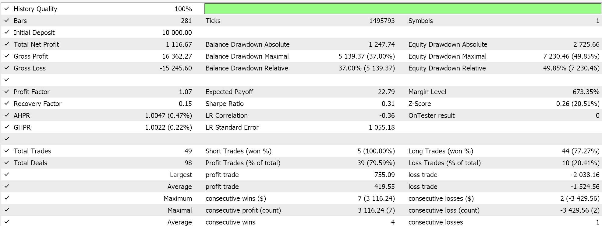
We get a promising forward walk, that however has a touch too few short trades when compared to the longs. More training should resolve this. This pattern Captures Early trend moves since the target is price crossing the MA, which could signal a trend shift and should lag less than 2 MAs crossing as we saw in pattern-0. It also filters out many false breakouts since the Stochastic is used as a confirmation, and this helps avoid premature trades.

This pattern also has its weaknesses and Limitations. First up, the lagging nature of the MA, especially when longer periods are used can make entries into trades sluggish. We use a period of 8 on the Daily time frame by default, but this is an optimisable parameter for the custom signal class, so readers can fine tune this to what works. Secondly, the Stochastic Oscillator is infamous for being very choppy, especially in ranging markets. This can lead to a lot of false confirmations. Also, in situations where an asset is already trending strongly, waiting for a price cross from the MA could result in a lot of missed early entries.

As far as optimising the indicator periods is concerned, a short MA in the sub 20 period range is bound to react faster to price changes than say a longer period in the 50 to 200 range. So users need to factor in the timeframe they are using to decide if they are looking for quick reactions, or they want stability, and more certainty before they accept changes.

Similarly for the stochastic, (5,3,3) does provide faster settings, but the generated signals are bound to be noisy. Slower settings of say (14,5,5) could be deemed more appropriate, but again this is something one should take into consideration together with the timeframe he is using. In the custom signal class that we are using for these tests, we have used a standard indicator period for the moving average and the stochastic Oscillator.  These are customisable but to illustrate if our MA period is N, then the stochastic Oscillator will be (N,3,3) and the slow or lagging MA will be 2 x N.

Volume spikes can also be used to further confirm MA crossovers or the strength of a breakout. Support and resistance levels can also be used to further enhance the pattern's reliability.

Moving Average Slope + Stochastic Trend Confirmation

This pattern focuses on trend direction through the use of MA slope while confirming momentum with the Stochastic. A buy Signal is when the moving average is sloping upward AND the Stochastic is over 50 and rising. The sell Signal is the reverse. With the moving average sloping downward, while the Stochastic would be below 50 and falling. This is how our ‘Get’ function retrieves an input vector that checks for these conditions:

else if(Index == 2)
{  if(C.GetData(T, 2, _c) >= 2 && CopyBuffer(M.Handle(), 0, T, 2, _ma) >= 2 && CopyBuffer(S.Handle(), 0, T, 2, _sto_k) >= 2)
   {  _v[0] = ((_ma[1] < _ma[0]) ? 1.0f : 0.0f);
      _v[1] = ((_sto_k[1] < _sto_k[0] && _sto_k[1] >= 50.0) ? 1.0f : 0.0f);
      _v[2] = ((_sto_k[1] > _sto_k[0] && _sto_k[1] <= 50.0) ? 1.0f : 0.0f);
      _v[3] = ((_ma[1] > _ma[0]) ? 1.0f : 0.0f);
   }
}

This is the first pattern of the 10 where we use the second Stochastic buffer aka %k. It's always lagging the main buffer (%d) and it's use here helps confirm the slope of this Oscillator. Once vectors of this data, across the year 2023 for EUR JPY, are exported to Python, we would train the simple network we listed above with the ‘Train' function also listed above. Testing or the cross validation would be performed by a function that is very similar to our ‘Train’ function above that we have labelled the ‘Test’ function. Its Python listing is as follows:

# Test function
def Test(model, test_loader, optimizer, loss_fn, epochs):
    device = T.device('cuda:0' if T.cuda.is_available() else 'cpu')
    model.to(device)
    
    with T.no_grad():
        test_loss = 0.0
        
        for batch_idx, (data, target) in enumerate(tqdm(test_loader, desc=f"Loss at {test_loss} in (Test)")):
            # Step 1: Ensure proper tensor dimensions
            data = data.view(-1, 1, feature_size)
            
            ...

            # Step 3: Move to device and forward pass
            data, target = data.to(device), target.to(device)
            optimizer.zero_grad()
            output = model(data)
            target = target.view(-1, 1, 1)
            #print(f"target: {target.shape}, plus output: {output.shape}")
            loss = loss_fn(output, target)
            test_loss += loss.item()

        test_loss /= len(test_loader)
        print(f"Test Loss: {test_loss:.4f}")

Comparative train and test loss scores are in line with what was shared above with patterns 0 and 1 and therefore will not be posted here. A forward walk for the year 2024 in MetaTrader's strategy tester presents us with the following report:

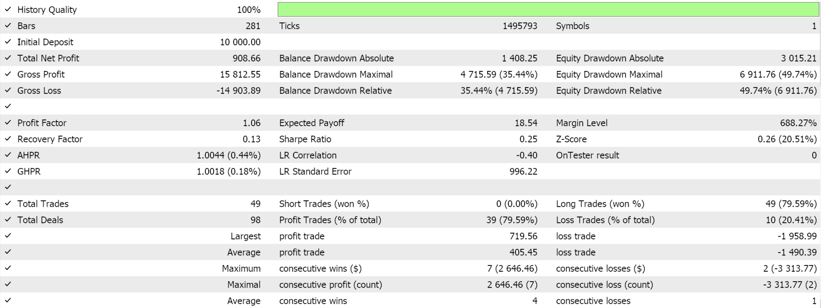
Our pattern is able to give a lob-sided walk, since only longs are open. Training on Larger data sets should solve this problem. Pattern-2 though, is a good filter for ranging markets. The MA slope makes certain trades are placed only when there is a clear trend. Confirmation of the trend strength is then done by the Stochastic Oscillator, since relative position to the 50 threshold validates momentum in the prevalent trend. Broadly there is also a reduction in lag since there is no waiting for MA crossovers as we have with the patterns above. This means this pattern bodes well for trend acceleration.

Its main weaknesses include slow reaction to trend reversals, since a moving average slope may take time to shift or change after a trend reversal. Also, the Stochastic in these situations can be prone to giving late signals. If a trend is already in play, waiting for the stochastic to confirm can lead to missed early entries. In general, also, this pattern is unsuited for Sideways markets given its strong dependency on trends.

Pairing it with additional filters such as the ADX (Average Directional Index) can help confirm strong trends. Also, checking for price action breakouts or pullbacks should improve accuracy. Practical Use Cases could include forex (which is what we are testing with here; or stocks since this pattern can help identify continuation trends after small retracements; or crypto & Commodities since it's useful in catching momentum induced moves in assets like Gold or Bitcoin.

MA Bounce with Stochastic Divergence

This pattern works by combining the dynamic support/resistance of Moving Average price bounces with momentum divergence from the Stochastic Oscillator to identify potential reversals 

before they happen. The buy signal is when price bounces off an upward sloping MA (which in this case would be acting as a support) and the stochastic Oscillator shows bullish divergence such that price makes a lower low while the oscillator makes a higher low. 

The sell Signal is where price rejects a downward sloping MA that is acting as resistance and the stochastic Oscillator indicates a bearish divergence where price makes a higher high but the Stochastic makes a lower high. Implementation in MQL5 and the definition of the input to the network that processes this pattern is handled as follows:

else if(Index == 3)
{  _v.Init(6);
   _v.Fill(0.0);
   if(C.GetData(T, 3, _c) >= 3 && CopyBuffer(M.Handle(), 0, T, 3, _ma) >= 3 && CopyBuffer(S.Handle(), 0, T, 3, _sto_k) >= 3)
   {  _v[0] = ((_c[2] > _c[1] && _c[1] < _c[0] &&  _c[0] < _c[2] && _ma[1] >= _c[1]) ? 1.0f : 0.0f);
      _v[1] = ((_sto_k[2] > _sto_k[1] && _sto_k[1] < _sto_k[0] && _sto_k[1] >= 40.0) ? 1.0f : 0.0f);
      _v[2] = ((_ma[2] > _ma[0]) ? 1.0f : 0.0f);
      _v[3] = ((_ma[2] < _ma[0]) ? 1.0f : 0.0f);
      _v[4] = ((_sto_k[2] < _sto_k[1] && _sto_k[1] > _sto_k[0] && _sto_k[1] <= 60.0) ? 1.0f : 0.0f);
      _v[5] = ((_c[2] < _c[1] && _c[1] > _c[0] &&  _c[0] > _c[2] && _ma[1] <= _c[1]) ? 1.0f : 0.0f);
   }
}

Train and test validation loss function scores are not very different from logs of the first 2 patterns, whose logs were shared. The test loss function is less than the loss function from the training at the first epoch, but it is still less than the loss function at the 10th epoch. A forward walk report on the year 2024, after training on the year 2023 is as follows:

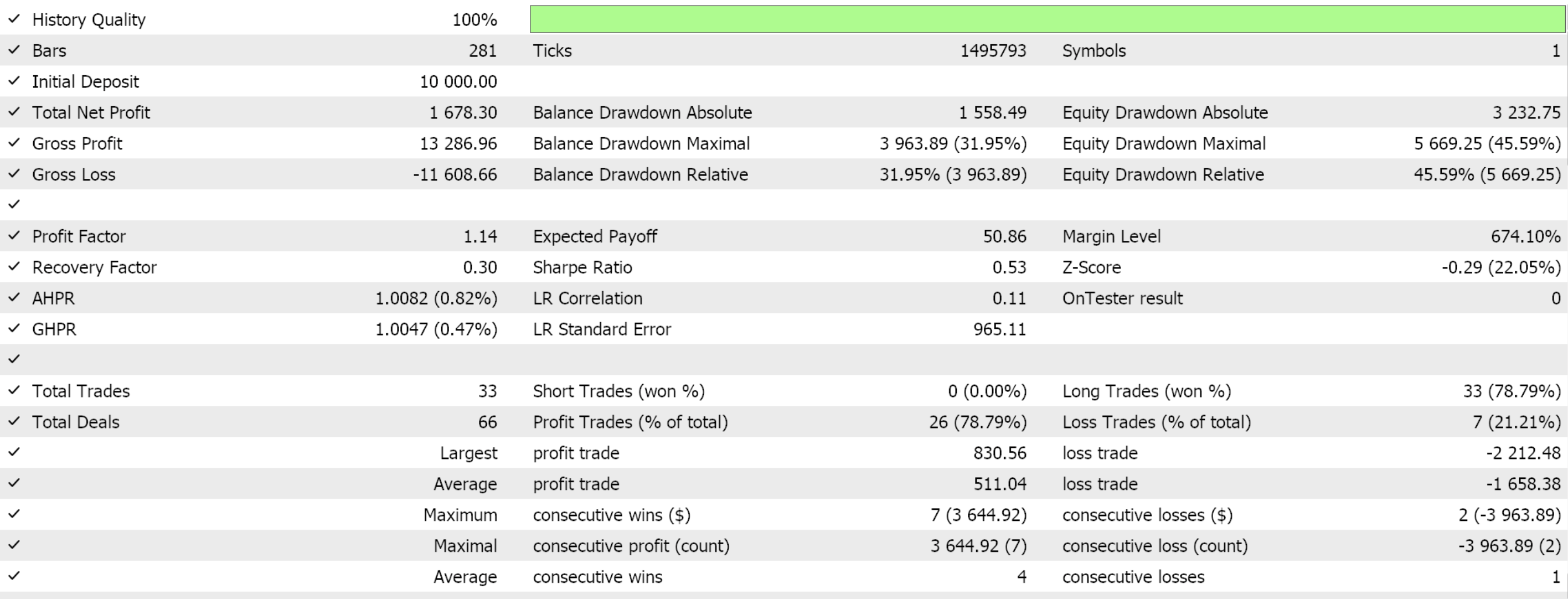
A positive forward walk is always a good sign, provided both long and short positions are opened in a balanced fashion. This is not the case here. However, Pattern-3 is good at early reversal detection, since the Stochastic divergence usually signals trend reversals before price reacts. It also avoids Chasing the Trend such that instead of entering late, traders get in near the dynamic support/ resistance level. It also works well in trending markets since the MA bounce would confirm the trend while the divergence warns of exhaustion.

Weaknesses and Limitations are its false signals when markets are trending strongly. This is because in these situations, divergence alone is often not sufficient for a reversal. Also, the lagging MA Effect since the MA bounce may not always align perfectly with divergence timing and the requirement for confirmation to improve accuracy are also drawbacks.

Pattern-3 can be optimized by pairing with candle stick patterns (such as pin bars or engulfing bars) at the MA level to strengthen the setup. Volume spikes can also be supplemented to confirm divergence.

MA Acting as Dynamic Support/Resistance + Stochastic Crossover

Our Pattern-4 strategy is a blend of trend following (when using MA for direction as well as support/ resistance) and momentum confirmation (which is done by checking for Stochastic cross-overs) in order to generate usable buy and sell signals.

The buy-signal is when price holds above an upward-sloping MA and the stochastic %K crosses above the %D. This bullish pattern helps ensure a number of key prerequisites for a long position. Firstly, it serves as trend confirmation, since an upward sloping MA ensures placed trades are in alignment with prevailing market direction.

Secondly, the crossover of the Stochastic does provide an entry timed to momentum. This is because a shift in momentum often confirms renewed buying pressure. Premature entries from any MA touch are avoided, since Stochastic crossover ensures momentum is present before buying. False Signals are therefore reduced. A potential drawback is it may miss early breakouts since it waits for both conditions, which results in slightly delayed entries.

The sell-signal is when price stays below a downward sloping moving average and the stochastic %K crosses below the %D. This similarly, like with its bullish counterpart, provides trend-confirmation, is a momentum-based entry or exit, there are no premature entries, and weak signals are filtered out. Potential Drawback is in choppy markets, price can breach MA before resuming downward descent. This is particularly key because for most trade symbols, their descents tend to be more volatile than their bullish trends. We implement this as follows in MQL5

else if(Index == 4)
{  if(C.GetData(T, 2, _c) >= 2 && CopyBuffer(M.Handle(), 0, T, 2, _ma) >= 2 && CopyBuffer(S.Handle(), 0, T, 2, _sto_k) >= 2 && CopyBuffer(S.Handle(), 1, T, 2, _sto_d) >= 2)
   {  _v[0] = ((_sto_k[1] < _sto_d[1] && _sto_k[0] > _sto_d[0]) ? 1.0f : 0.0f);
      _v[1] = ((_ma[1] < _c[1] && _ma[0] < _c[0] && _ma[1] < _ma[0]) ? 1.0f : 0.0f);
      _v[2] = ((_ma[1] > _c[1] && _ma[0] > _c[0] && _ma[1] > _ma[0]) ? 1.0f : 0.0f);
      _v[3] = ((_sto_k[1] > _sto_d[1] && _sto_k[0] < _sto_d[0]) ? 1.0f : 0.0f);
    }
}

We batch the input vector to the network processing this pattern into a 4-sized dimension. As shown on earlier patterns above, this vector can be made more explicit by having each of the arguments within a condition outlined as part of the inputs. A forward walk for the network trained on just pattern-4 gives us the following results:

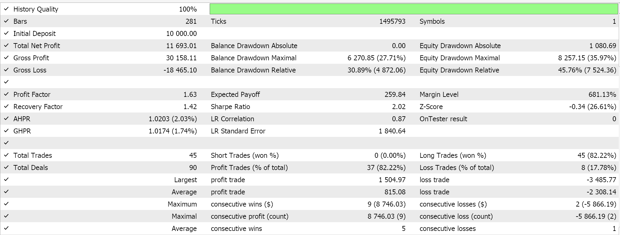
This pattern should be okay in trend-following markets, however it is bound to struggle in range bound scenarios. Though we have a favourable forward walk, testing on Larger data sets is important to ensure we can place both long and short trades, not just the longs as reported above.

Stochastic Overbought/Oversold Reversal Near MA

Pattern-5 brings together trend-following with the MA as a Dynamic support/ resistance and momentum -reversal with the Stochastic. The buy Signal is when the Stochastic crosses above the 20 threshold while price is being supported by the MA. This pattern provides dynamic support validation, since the MA acts as a support zone, ensuring that price is bouncing within an existing uptrend. The Stochastic crossing above 20 also signals that bearish momentum is weakening and buyers are coming into the market. The use of two indicators not only avoids premature entries, but is also a high probability setup. The Potential Drawback is that in strong downtrends, price may temporarily hold at the MA before breaking lower.

The sell Signal is when Stochastic crosses below 80 while price is close to the resistance of a downward sloping moving average. This also acts as dynamic resistance validation since MA performs as a resistance zone which serves as proof that price has failed to rise higher. The overbought Reversal Confirmation signals to waning bullish momentum and that sellers are coming in. Once again, the dual indicator use avoids premature exits/ entries and also filters out weak pullbacks. A Potential Drawback to pattern-5's bearish signal is that in strong downtrends, price may consolidate above MA before breaking lower, which could lead to late exits or missed pips.

We implement this as follows in MQL5:

else if(Index == 5)
{  if(C.GetData(T, 3, _c) >= 3 && CopyBuffer(M.Handle(), 0, T, 3, _ma) >= 3 && CopyBuffer(S.Handle(), 0, T, 2, _sto_k) >= 2)
   {  _v[0] = ((_sto_k[1] < 20.0 && _sto_k[0] > 20.0) ? 1.0f : 0.0f);
      _v[1] = ((_c[2] > _c[1] && _c[1] < _c[0] && _c[1] >= _ma[1]) ? 1.0f : 0.0f);
      _v[2] = ((_c[2] < _c[1] && _c[1] > _c[0] && _c[1] <= _ma[1]) ? 1.0f : 0.0f);
      _v[3] = ((_sto_k[1] > 80.0 && _sto_k[0] < 80.0) ? 1.0f : 0.0f);
   }
}

Our MQL5 pattern implementations for this article aim to set or define an input vector for a neural network. We define these input vectors as being simply a collection of 0s and 1s, where a 1 is if a particular long or short condition is met. The indices for long and short conditions are separate, which technically means it's not possible to have an input vector that is filled with 1s, since the long and short conditions always mirror each other.

Also, the condition at each index can be further detailed or lengthened by having each of the arguments in the condition taking up their own index. This would lead to much longer input vectors, however we have not explored it. Since we are testing and training on the year 2023, a forward walk is this for the year 2024. It gives us the following report:

We are able to forward walk with Pattern-5, with one caveat. Only long trades were placed! This is mostly down to training on limited/ small data sets such that the network outputs get skewed to that small sample. Training with larger data sets should remedy this.

Golden Cross/Death Cross + Stochastic Confirmation

Pattern-6 uses the golden-cross/ death-cross where the shorter period MA crosses the lagging MA and momentum is also verified by the Stochastic crossing the 50 level. The buy Signal is the Golden Cross of the shorter period MA crossing from below to above the longer period MA, while the Stochastic is above 50 and rising. The sell Signal is the death-cross with shorter period MA crossing the longer period from above to close below it, while the Stochastic is below 50 and falling. We set the inputs for the network of pattern-6 as follows:

else if(Index == 6)
{  if(CopyBuffer(M.Handle(), 0, T, 2, _ma_lag) >= 2 && CopyBuffer(M.Handle(), 0, T, 2, _ma) >= 2 && CopyBuffer(S.Handle(), 0, T, 2, _sto_k) >= 2 && CopyBuffer(S.Handle(), 0, T, 2, _sto_d) >= 2)
   {  _v[0] = ((_ma_lag[1] > _ma[1] && _ma_lag[0] < _ma[0]) ? 1.0f : 0.0f);
      _v[1] = ((50.0 <= _sto_d[0] && _sto_k[0] > _sto_d[0]) ? 1.0f : 0.0f);
      _v[2] = ((50.0 >= _sto_d[0] && _sto_k[0] < _sto_d[0]) ? 1.0f : 0.0f);
      _v[3] = ((_ma_lag[1] > _ma[1] && _ma_lag[0] < _ma[0]) ? 1.0f : 0.0f);
   }
}

In our used source the handle ‘_ma’ is the shorter period moving average for which in our training we have assigned the period 8. The longer period average uses the handle ‘_ma_lag' and its period is twice that of the shorter at a length of 16. A forward walk on the year 2024 after training on the year 2023 gives us this report:

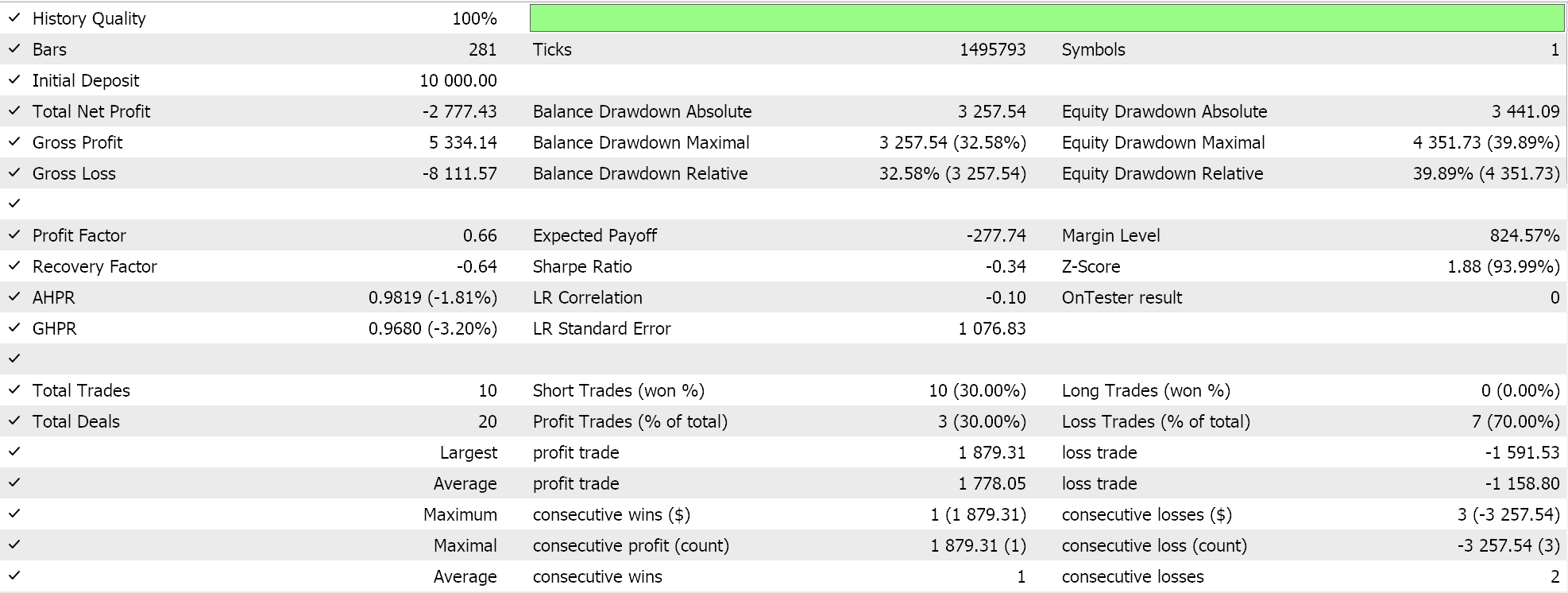
Pattern-6 fails its walk not just on profitability but on a balance between longs and shorts. This can be taken further though with extensive training and testing before it is written off.

Stochastic Extreme Reversal + MA Trend Confirmation

Pattern 7 uses Stochastic inflection at extreme levels together with relative position of price to MA to define its entry signals. Buy Signal is when Stochastic is below 10 and starts turning up while price is above an upward sloping moving average. Sell Signal is a downturn at a level over 90 when price is below a down sloping moving average. We map this as follows to a network from MQL5:

else if(Index == 7)
{  if(C.GetData(T, 2, _c) >= 2 && CopyBuffer(M.Handle(), 0, T, 2, _ma) >= 2 && CopyBuffer(S.Handle(), 0, T, 3, _sto_k) >= 3)
   {  _v[0] = ((_ma[0] > _ma[1] && _c[0] > _ma[0]) ? 1.0f : 0.0f);
      _v[1] = ((_sto_k[0] > _sto_k[1] && _sto_k[1] < _sto_k[2] && _sto_k[2] <= 10.0) ? 1.0f : 0.0f);
      _v[2] = ((_sto_k[0] < _sto_k[1] && _sto_k[1] > _sto_k[2] && _sto_k[2] >= 90.0) ? 1.0f : 0.0f);
      _v[3] = ((_ma[0] < _ma[1] && _c[0] < _ma[0]) ? 1.0f : 0.0f);
   }
}

We strictly use the %K handle for the stochastic here and all we are doing is checking for the n-shaped turn for the bullish conditions or u-shape reversal for the bearish when at extreme levels. A Forward walk, gives us the following report:

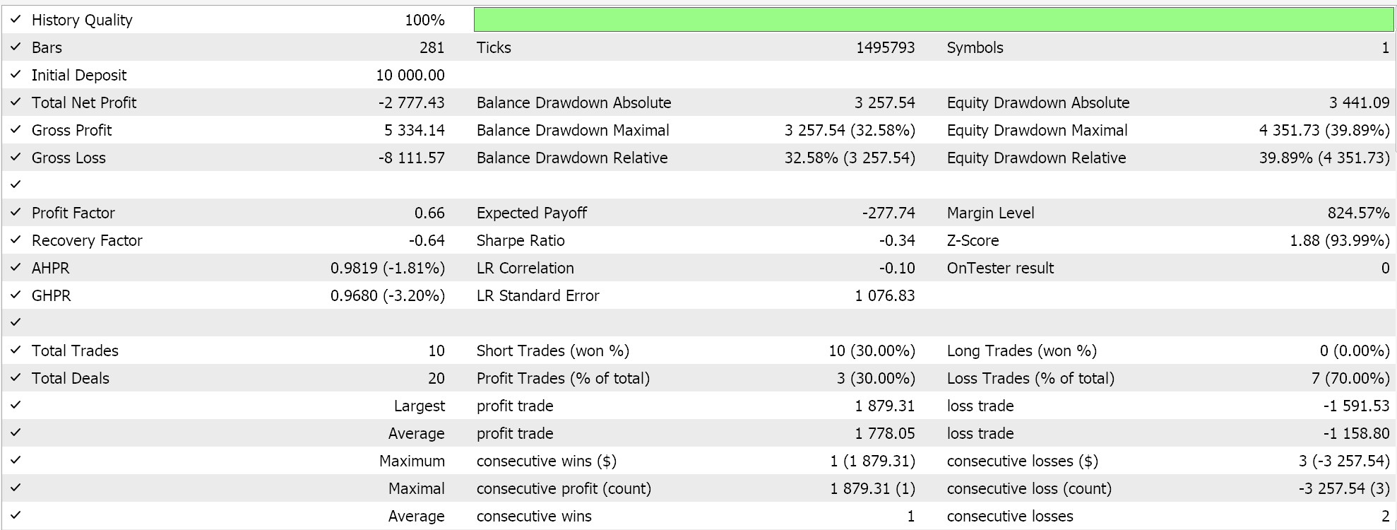
From our results above, this pattern also cannot forward walk for a year based on prior year testing. And it only places short trades. Placing one-sided trades in a forward walk can be concerning. Since our output is a scalar float value in the 0.0 - 1.0 range, this means all forecasts were sub 0.5. Testing/ training on larger data sets is important in rectifying this.

Stochastic Breakout with MA Confirmation

Our penultimate pattern, Pattern-8 combines the 50 stochastic threshold with price-MA crossings. A buy Signal is when there is a pickup in momentum as signalled by the Stochastic Oscillator crossing the 50 threshold from below to close above it, while simultaneously price crosses MA in similar fashion to also close above it. Sell is the inverse, with Oscillator crossing below 50 while price breaks through MA support. This is bound to be a pattern that does not generate a lot of trades, if, we were to apply it similarly to what we were doing in previous articles. However, we are now checking separately for MA and Stochastic conditions for both bullish and bearish signals. This is done as follows in MQL5:

else if(Index == 8)
{  if(C.GetData(T, 2, _c) >= 2 && CopyBuffer(M.Handle(), 0, T, 2, _ma) >= 2 && CopyBuffer(S.Handle(), 0, T, 2, _sto_k) >= 2 && CopyBuffer(S.Handle(), 1, T, 2, _sto_d) >= 2)
   {  _v[0] = ((_c[1] < _ma[1] && _c[0] > _ma[0]) ? 1.0f : 0.0f);
      _v[1] = ((_sto_k[1] < 50.0 && _sto_k[0] > 50.0) ? 1.0f : 0.0f);
      _v[2] = ((_sto_k[1] > 50.0 && _sto_k[0] < 50.0) ? 1.0f : 0.0f);
      _v[3] = ((_c[1] > _ma[1] && _c[0] < _ma[0]) ? 1.0f : 0.0f);
   }
}

Our input vector for the pattern-8 network is now more likely to have or register at least one of the bullish or bearish conditions, and this helps with the training but also adaptability when it comes to deploying the network. This is because it will, in addition to processing both indicators, it would give forecasts if only one of them registers the target patterns. A forward walk gives us the following:

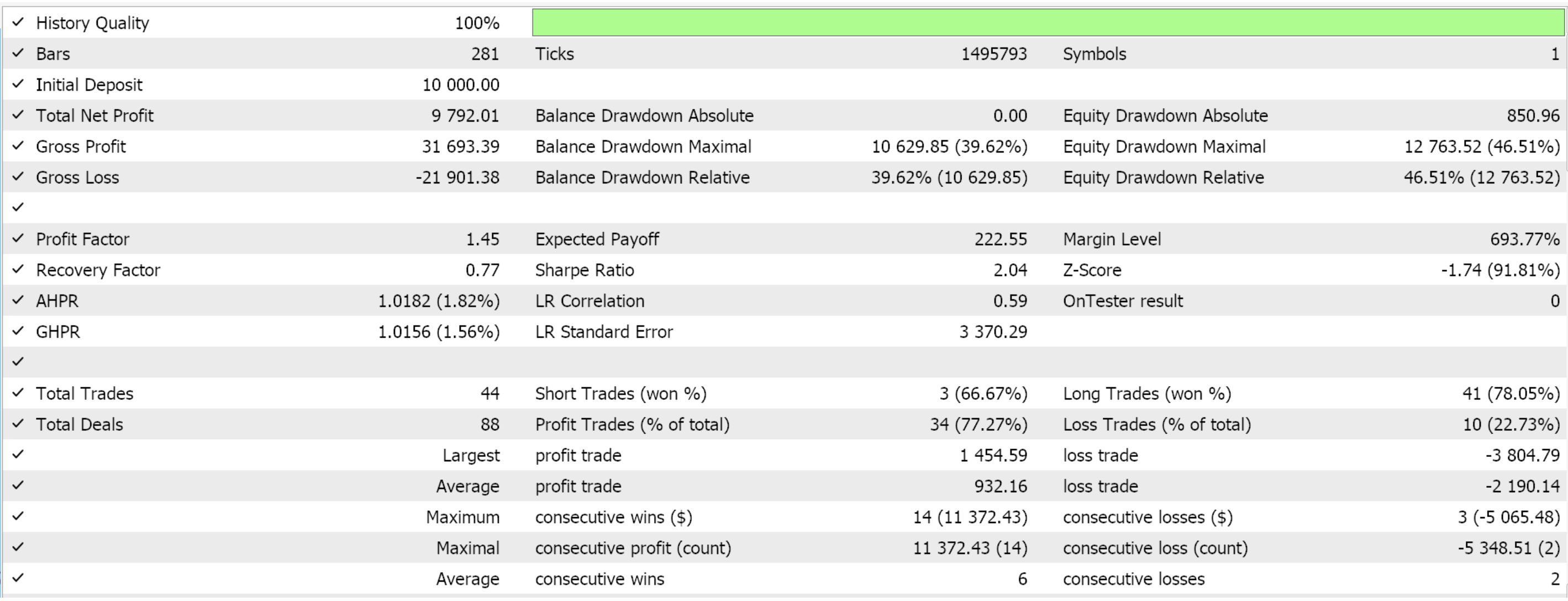
It seems this pattern is able to walk, which is encouraging. Key caveats are worth mentioning here. First, these test runs are done with price targets (take-profits) and no stop loss. It's true, stop loss never guarantees exit price, but one needs some strategy in place to cater for unsuccessful trades. Secondly, we trained on the recent year and tested on the subsequent one, which is relatively a short testing window. Longer test periods with good quality broker data are often preferred.

Moving Average Squeeze with Stochastic Breakout

Our final pattern, 10, leverages moving average compression to sense low-volatility conditions together with Stochastic momentum to time breakouts from these conditions. The buy Signal is when two MAs a shorter period and a longer period squeeze together for an extended period and after which a pickup in momentum is registered as per the Stochastic moving sharply through 50. A bearish signal also registers the same conditions with the first change being the bullish squeeze has the shorter MA above the longer MA while for the sell Signal this is reversed, and the stochastic for the sell sharply drops through the 50 level (instead of rising)

We retrieve the network input vector from MQL5 as follows:

else if(Index == 9)
{  if(CopyBuffer(M.Handle(), 0, T, 3, _ma) >= 3 && CopyBuffer(M_LAG.Handle(), 0, T, 3, _ma_lag) >= 3 && CopyBuffer(S.Handle(), 0, T, 2, _sto_k) >= 2)
   {  _v[0] = ((_ma_lag[0] < _ma[0] && fabs(fabs(_ma_lag[2] - _ma[2]) - fabs(_ma_lag[0] - _ma[0])) <= fabs(_ma[2] - _ma[0])) ? 1.0f : 0.0f);
      _v[1] = ((_sto_k[1] <= 45.0 && _sto_k[0] >= 55.0) ? 1.0f : 0.0f);
      _v[2] = ((_sto_k[1] >= 55.0 && _sto_k[0] <= 45.0) ? 1.0f : 0.0f);
      _v[3] = ((_ma_lag[0] > _ma[0] && fabs(fabs(_ma_lag[2] - _ma[2]) - fabs(_ma_lag[0] - _ma[0])) <= fabs(_ma[2] - _ma[0])) ? 1.0f : 0.0f);
   }
}

And its walk forward results are as follows:

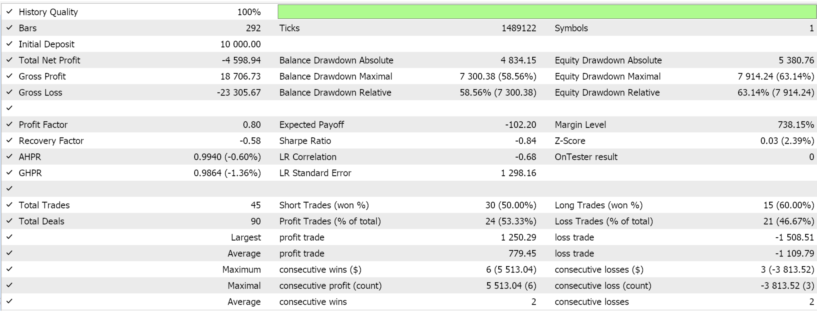
Pattern-9 also it seems does not have legs, despite being able to place both long and short trades. On an equal weighted basis it should not be studied further since we have some patterns above that had favourable walks, but this decision is up to the trader and how much more testing he is willing to do.

Conclusion

We have not got into combining patterns or cherry-picking different patterns to come up with a unified system. This is something that is bound to be dangerous, as we've observed in past articles, especially the last one. Using multiple patterns at ago requires the trader to be versed with them because they can cancel each other's trades. If magic numbers are used in tracking, this could help but still challenges could remain with margin limits. In the next piece, we'll look at how reinforcement-learning can build on what we have got here.

File	Description
57_0.onnx	pattern-0 network
57_1.onnx	pattern-1 "
57_2.onnx	pattern-2 "
57_3.onnx	pattern-3 "
57_4.onnx	pattern-4 "
57_5.onnx	pattern-5 "
57_6.onnx	pattern-6 "
57_7.onnx	pattern-7 "
57_8.onnx	pattern-8 "
57_9.onnx	pattern-9 "
SignalWZ_57.mqh	Signal Class File
57_X.mqh	Signal File for processing network inputs
wz_57.mq5	Included to show used files in assembling Expert Advisor