MQL5 Wizard Techniques you should know (Part 55): SAC with Prioritized Experience Replay

The growing complexity of neural network models is driven by our ability to process vast amounts of data. Traditional machine learning struggles with efficiency, while neural networks, exemplified by platforms like DeepSeek, Grok, and ChatGPT, offer powerful solutions.

However, training these models presents challenges, especially with limited historical data. Overfitting is a major concern, as models risk learning noise instead of meaningful patterns. Traditional training often prioritizes minimizing loss functions, which can lead to poor generalization.

Reinforcement learning (RL) addresses this by balancing exploitation (optimizing weights) and exploration (testing alternatives). Techniques like Prioritized Experience Replay (PER) enhance learning efficiency, mitigating data scarcity issues seen in fields like trading, where monthly economic data points are limited.

Key RL considerations include designing an effective reward function, selecting the right algorithm, and deciding between value-based (e.g., Q-Learning, DQN) and policy-based methods (e.g., PPO, TRPO). Actor-Critic approaches (e.g., A3C, SAC) balance stability and efficiency. On-policy methods (PPO, A3C) ensure stable learning, while off-policy methods (DQN, SAC) maximize data efficiency.

RL’s adaptability makes it a valuable addition to machine learning pipelines, complementing traditional approaches. When training complex models with limited data, prioritizing weight updates over loss minimization fosters better generalization and robustness.

Prioritized Experience Replay

Prioritized Experience Replay (PER) buffers and typical Replay Buffers (for random sampling) are both used in RL with off-policy algorithms like DQN and SAC because they allow for storing and sampling of past experiences. PER does differ from a typical replay buffer in how past experiences are prioritized and sampled. 

With the typical replay buffer, experiences are sampled uniformly and at random meaning any of the past experiences has an equal probability of being selected regardless of its importance or relevance to the learning process. With PER, past experiences are sampled based on their ‘priority’, a. property that is often quantified by the magnitude of the Temporal Difference Error. This error serves as a proxy for learning potential. Each experience gets assigned a value of this error and experiences with high values get sampled more frequently. This prioritization can be implemented using a proportional or rank based approach.

Typical replay buffers also do not introduce or use any biases. PER does and this could unfairly skew the learning process which is why, to correct this PER uses importance sampling weights to adjust the impact of each sampled experience. Typical replay buffers are thus more sample efficient since they are accomplishing way fewer things in the background as opposed to PER. On the flip side PER provides more focused and constructive learning which the typical buffers do not.

It goes without saying therefore that implementing a PER would be more complex than a typical replay buffer; however why this is emphasized here is because PER requires an additional class, to maintain the priority queue often referred to as the ‘sum-tree’. This data structure allows for a more efficient sampling of experiences based on their priority. PER tends to lead to faster convergence and better performance as it focuses on experiences that are more informative or challenging for the agent.

Implementation in Model

Our PER class, in Python uses initialization that validates it's constructor parameters, specifically the mode parameter. I could be mistaken but I think this is something that cannot be done out of the box with C/ MQL5. We declare this __init__ function as follows:

        def __init__(self, capacity, alpha=0.6, beta=0.4, beta_increment=0.001, mode='proportional'):
                self.capacity = capacity
                self.alpha = alpha
                self.beta = beta
                self.beta_increment = beta_increment
                self.mode = mode

                if mode == 'proportional':
                        self.tree = SumTree(capacity)
                elif mode == 'rank':
                        self.priorities = []
                        self.data = []
                else:
                        raise ValueError("Invalid mode. Choose 'proportional' or 'rank'.")

With the class declared one of the important functions it should include is a method to add experiences to the buffer. We implement this as follows: 

    def add(self, error, sample):
        p = self._get_priority(error)
        if self.mode == 'proportional':
            self.tree.add(p, sample)
        elif self.mode == 'rank':
            heapq.heappush(self.priorities, -p)
            if len(self.data) < self.capacity:
                self.data.append(sample)
            else:
                heapq.heappop(self.priorities)
                heapq.heappush(self.data, sample)

Note that in this addition of experiences the mode of sampling is Key since if we are selecting experiences based on the proportion of the error, we merely append them to the sum-tree, but if we are choosing based on the ranking of the error magnitude, we use an imported module heapq that we update with this sample as indicated above. The sum-tree class therefore is used in the proportion sampling and not the rank. This is how it's implemented:

class SumTree:
    def __init__(self, capacity):
        self.capacity = capacity
        self.tree = np.zeros(2 * capacity - 1)
        self.data = np.zeros(capacity, dtype=object)
        self.write = 0
        self.n_entries = 0

    def _propagate(self, idx, change):
        parent = (idx - 1) // 2
        self.tree[parent] += change
        if parent != 0:
            self._propagate(parent, change)

    def _retrieve(self, idx, s):
        left = 2 * idx + 1
        right = left + 1

        if left >= len(self.tree):
            return idx

        if s <= self.tree[left]:
            return self._retrieve(left, s)
        else:
            return self._retrieve(right, s - self.tree[left])

    def total(self):
        return self.tree[0]

    def add(self, p, data):
        idx = self.write + self.capacity - 1

        self.data[self.write] = data
        self.update(idx, p)

        self.write += 1
        if self.write >= self.capacity:
            self.write = 0

        if self.n_entries < self.capacity:
            self.n_entries += 1

    def update(self, idx, p):
        change = p - self.tree[idx]
        self.tree[idx] = p
        self._propagate(idx, change)

    def get(self, s):
        idx = self._retrieve(0, s)
        data_idx = idx - self.capacity + 1
        return (idx, self.tree[idx], self.data[data_idx])

With this key class defined, the other crucial component of this is the sample function itself which is part of the PER class. 

def sample(self, batch_size):
        batch = []
        idxs = []
        segment = self.tree.total() / batch_size if self.mode == 'proportional' else len(self.data) / batch_size
        priorities = []

        self.beta = np.min([1., self.beta + self.beta_increment])

        for i in range(batch_size):
            a = segment * i
            b = segment * (i + 1)

            if self.mode == 'proportional':
                s = random.uniform(a, b)
                (idx, p, data) = self.tree.get(s)
                priorities.append(p)
                batch.append(data)
                idxs.append(idx)
            elif self.mode == 'rank':
                idx = random.randint(0, len(self.data) - 1)
                priorities.append(-self.priorities[idx])
                batch.append(self.data[idx])
                idxs.append(idx)

        sampling_probabilities = np.array(priorities) / self.tree.total() if self.mode == 'proportional' else np.array(priorities) / sum(self.priorities)
        is_weights = np.power(len(self.data) * sampling_probabilities, -self.beta)
        is_weights /= is_weights.max()

        return batch, idxs, is_weights

Once again the mode of sampling whether proportional based or rank based is a key consideration here. These two approaches assign the priorities of each experience, while considering the TD error, with a nuanced difference. Magnitude of the TD error and rank of the TD error. The TD error is effectively the difference between an experiences output and the actual or target value. It is never used in its raw state to weight the experiences but rather is converted to a priority value as shown in this listing:

def _get_priority(self, error):
        return (error + 1e-5) ** self.alpha

It is this priority value whose magnitude (for proportion sampling) or rank (for rank sampling) that gets used in selecting experiences to train the model. PER was introduced by Shaul et al in 2015.  Higher priority experiences are sampled more frequently, improving sample efficiency and learning speed in the RL environment. The priorities do get updated after learning. The importance sampling weights are engaged to correct bias brought in from the non uniform priority based sampling. This is indicated in the sample function of the PER class above. Let's delve into these two modes of sampling.

Proportional Prioritization

As mentioned above priorities are directly proportional to the Temporal Difference Error (∣δ∣). The priority for an experience i would therefore be computed as:

pi=∣δi∣+ϵ

Where ϵ, which is greater than zero, is a small constant that ensures all experiences do not have a zero priority. The sampling probability for the experience would therefore be:

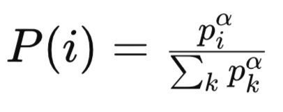
Where:

• is the **priority** of the  i -th experience in the replay buffer. The priority is typically based on the magnitude of the temporal difference (TD) error for that experience. Experiences with larger TD errors are considered more important and are assigned higher priorities.

• This is a hyperparameter that controls the degree of prioritization. When (  α = 0 ), all experiences are sampled uniformly (no prioritization). When ( α = 1 ), sampling is fully based on the priorities.

• This is the normalization term, which ensures that the probabilities sum to 1. It sums the priorities of all experiences in the replay buffer, raised to the power of ( α).

• This is the probability of sampling the ( i )-th experience. It is proportional to the priority of the experience (Piα), normalized by the sum of all priorities raised to the power of ( α).

A Sum Tree or a data structure of similar form can then be used to efficiently sample the experiences I. proportion to piα. The sampling distribution with proportional prioritization is continuous and directly tied to the magnitude of TD errors. Experiences with high TD errors tend to have significantly high priorities which leads to a heavy tailed distribution.

This could lead to some experiences being too frequently sampled (a major concern if their TD errors were outliers) and others being rarely sampled because their errors are small. Sensitivity to training errors can vary across tasks of the training phases but there is a vulnerability for proportional prioritization to outliers in TD errors as large values can dominate the sampling distribution.

For instance consider a scenario where one experience had an output to target gap of 1000 while the others had theirs at 1, clearly this large value will be sampled often disproportionately. This trait can lead to overfitting to noisy or outlier experiences, particularly in data environments with high variance in rewards or Q-values. A possible mitigation measure for this could be clipping or normalization of the TD error. For instance:

pi=min⁡(∣δi∣,δmax)+ϵ

Where in essence an experience's priority is set to the minimum between its own TD error, and the highest TD error of all experiences within the sampled segment plus a small non zero value, epsilon. The operational time complexities when dealing with a sum-tree are straight forward when Computing the priority for each experience as they come to O(1) per experience. The sampling and updating of priorities comes to O(log n) per operation where n is the buffer size. With no additional overhead for sorting and ranking this makes it computationally efficient for updates.

Proportional Prioritization (PP) can foster unstable training in cases where TD errors vary significantly across training phases since the sampling distribution would be changing rapidly. It is also sensitive to hyperparameters so the choices for alpha and epsilon need to be made carefully to balance exploration and exploitation. PP may converge faster for tasks with ‘well-behaved’ errors which is indicative of the learning value, its bound to struggle in noisy and non-stationary environments.

PP is suitable for tasks when TD errors are well behaved and directly indicative of learning potential/ value. Being very effective in environments with low noise and stable Q-values where TD errors are directly proportional to important experiences. Examples of this include Atari games with stable reward structures, and continuous control tasks with smooth value functions.

PP's importance sampling weights do tend to vary because of heavy tailed sampling distribution. Experiences with low priority weights and therefore low P(i) values (i.e. probability of sampling experience i) and this leads to large wi weights (adjustment weights meant to correct for bias). This setup has the potential for an unintended consequence of amplifying gradients and destabilizing training. This means therefore that beta needs to also be tuned carefully to strike a balance between bias correction and stability.

To sum up PP, it is suited when TD errors are well behaved and correlate with the learning value; the data environment has low noise and stable Q-values; and computational efficiency is critical meaning sorting and ranking overheads are not acceptable. The fine tuning of the hyperparameters alpha, beta, and epsilon can help with handling outliers and managing instability.

Rank-based Prioritization

With this mode, priorities are based on ranks index values of the TD error in the sorted list of TD errors. The rank of an experience  i is set by sorting all experiences by the magnitude of the Temporal Difference Error in descending order. Why descending order, because intuitively such a list interprets to the importance of an experience. The higher up on the list, the more important an experience is. Secondly, from a computation stand point, it makes sense to have the experiences that will be referred to the most at the lower indices within a heap as the algorithm does not have to traverse the entire heap to get to the experiences meant to perform most of the training. The priority of experience i is usually computed as:

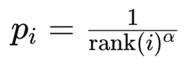
where:

- rank(i) is the rank of the  i -th experience.

- alpha  is a hyperparameter that controls the strength of prioritization.

The sampling probability for the experience uses a formula similar to what we have already covered above in proportional prioritization.

With Rank-Based Prioritization (RP) the sampling distribution is discrete and based on ranks. This tends to make it less sensitive to the absolute Scale of TD errors. Experiences are chosen based on their rank rather that error magnitude. This leads to a more uniform distribution when sampling given that the difference in prioritization between the experiences is almost “standardized” since it is controlled by the experiences respective ranking (i. e. 1/1, ½, ⅓, etc..). Furthermore RP is less prone to overfitting outliers since the highest assigned priority to any experience is fixed at 1/1 regardless of its TD error magnitude. This robustness though, is overshadowed by under sampling of experiences with very high TD errors if the rank-based priority function decays too quickly.

However, besides the risk in under sampling key experiences, the major drawback for RP remains computational Complexity. Sorting an entire buffer to determine the ranks is an operational computation complexity of magnitude O(nlogn) for an entire buffer of size n. In practice this sorting can be avoided by maintaining a sorted data structure (such as a binary search tree or a heap) for the TD errors but updates still require O(logn) operational computations per experience. Sampling and updating remain at O(logn) as was the save with proportional based sampling. In summation then RP has significantly higher computational overhead when compared to PP.

When training RP is more stable since the sampling distribution is less sensitive to changes in TD error magnitudes. It also tends to provide consistent sampling probabilities over time given that ranks are relative and less affected by noise and outliers. It may converge more slowly for tasks where absolute TD errors are crucial/ highly informative to the training process since it does not prioritize high magnitude errors as aggressively. It's also slightly easier to tune (adjusting hyperparameters) this is because the rank based priority function is less sensitive to scale.

RP is suitable in sparse reward environments or for tasks that have delayed rewards or high reward variance. RP is a preferred mode where stability and balanced sampling are critical even if convergence may be slow.

Both PP and RP introduce a bias given their non uniform sampling methods and as already mentioned and shown in the sampling method in the source above. The basic formula for this is:

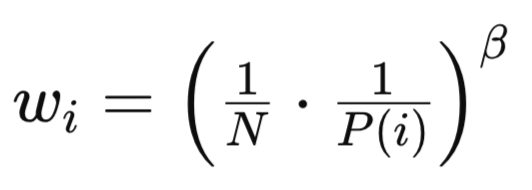
where:

- N is the total number of experiences in the replay buffer.

- P(i) is the probability of sampling the i -th experience.

- beta (β∈[0,1]) is a hyperparameter that controls the strength of the importance sampling correction.

Despite having similar formulae, RP and PP wi weights do differ in key aspects. For RP, the importance sampling weights are more uniform given that the distribution is less skewed. This lower variance in wi values leads to more stable training and less sensitivity to beta. Also, the bias correction is easier to manage since the rank-based distribution is inherently more balanced.

Testing Signal Class

If we use the listed code above and modify the SAC model code of the last article by having a PER instead of a typical/ simple replay buffer, we would be in a position to train the model and export a network with its weights as an ONNX file. We covered how this export can be managed in that last article, and there are Guidance notes here on how to also export an ONNX model from python. ONNX models are used by MQL5 by having them embedded as resources at compilation. 

On the MQL5 side in the IDE, our custom signal class which strictly speaking does not differ from what we had in the last SAC article, should be assembled by the MQL5 wizard and for new readers there are guides here and here on how to do that. None cross-validated test runs for USD JPY on the daily time frame for the year 2023 do present us with the following report:

Going forward though, cross validation with models in Python can be done very efficiently so perhaps it is something I will start to incorporate in these articles I the future. However, as always past performance does not guarantee future results and the reader is always invited to undertake his own extra diligence before choosing to use or deploy any of the systems that are shared here.

Conclusion

We have revisited the case for reinforcement learning by reiterating why in today’s setting of complex models and constrained historic test data, it is very important to put the process of arriving at the suitable network weights above and notional low-loss function scores. Process matters. And to thus end we have highlighted an alternative replay buffer for reinforcement learning, the Prioritized Experience Replay buffer as a buffer that not only keeps at hand recent experiences for sampling when training, but that also samples from this buffer in proportion to how relevant or by how much the network has to learn from the sampled experience.

File	Description
wz_55.mq5	Wizard  assembled Expert advisor with Header showing used files
SignlWZ_55.mqh	Custom Signal Class File
USDJPY.onnx	ONNX Network File