Portfolio Risk Model using Kelly Criterion and Monte Carlo Simulation

Introduction

For decades, traders have been using the Kelly Criterion formula to determine the optimal proportion of capital to allocate to an investment or bet to maximize long-term growth while minimizing the risk of ruin. However, blindly following Kelly Criterion using the result of a single backtest is often dangerous for individual traders, as in live trading, trading edge diminishes over time, and past performance is no predictor of future result. In this article, I will present a realistic approach to applying the Kelly Criterion for one or more EA's risk allocation in MetaTrader 5, incorporating Monte Carlo simulation results from Python.

The Leverage Space Trading Model Theory

The Leverage Space Trading Model (LSTM) is a theoretical framework used primarily in the context of financial markets and asset management. It integrates the concept of leverage, which refers to using borrowed funds to amplify potential returns, with a more dynamic and space-oriented approach to modeling market behavior. 

LSTM utilize the Kelly criterion to calculate the percentage of portfolio to risk per trade for a single strategy is

• L: leverage factor
• p:probability of success
• u:leveraged gain ratio
• l:leveraged loss ratio

Given a backtest result, we can obtain the variable value by the following formulas.

Let's say you're trading with 2:1 leverage. Assume the following:

• The probability of a successful trade (p) = 0.6 (60% chance of winning).
• The expected return (u) = 0.1 (10% gain without leverage, so leveraged 2:1 = 20% gain).
• The expected loss (l) = 0.05 (5% loss without leverage, so leveraged 2:1 = 10% loss).

Substitute into the Kelly formula:

So, the optimal fraction of your capital to risk on this trade would be 8% of your total capital.

After applying this formula to one of your own EAs, I believe you'll inevitably feel a sense of discomfort seeing how much risk you should've taken per trade. Indeed, this formula assumes that your future results will be just as good as your backtest, which is unrealistic. That's why, in the industry, people normally apply fractional Kelly to their risk, meaning that they divide the value by some integer to decrease their risk and allow room for future adversity.

Now we have to answer: what fraction should be chosen so that traders feel comfortable risking, while still maximizing their expected return per trade?

From the book The Leverage Space Trading Model by Ralph Vince, it was concluded through a stochastic optimization process that the return expectation function is convex, regardless of the dimension. This means that the optimal expected return has a single solution, and the expectation decreases continuously as the f* value moves away from the optimal solution.

This implies that because live trading is not as ideal as backtesting, we expect the real f* that will maximize our return to be smaller than the f* calculated from the Kelly formula. Therefore, all we have to do is increase our allocated risk to the highest level we can tolerate, while making sure it’s still smaller than the Kelly risk.

Usually, a trader's tolerance level is measured by the maximum drawdown they can endure. I will assume a reasonable tolerance level is 30% maximum drawdown for the rest of the article.

Applying leveraged risk in MQL5

To apply leveraged risk in MQL5, first we declare the risk percentage as a global variable. In this case, we risk 2% per trade.

input double risk = 2.0;

Next, we'll write a function to calculate the lot volume based on the stop loss in the current price unit. For instance, if the stop loss is set at a price of 0, the stop loss points will directly correspond to the current price, and the trade’s outcome will reflect the exact movement of the underlying asset.

//+------------------------------------------------------------------+
//| Calculate the corresponding lot size given the risk              |
//+------------------------------------------------------------------+
double calclots(double slpoints)
{
   double riskAmount = AccountInfoDouble(ACCOUNT_BALANCE) * risk / 100;

   double ticksize = SymbolInfoDouble(_Symbol, SYMBOL_TRADE_TICK_SIZE);
   double tickvalue = SymbolInfoDouble(_Symbol, SYMBOL_TRADE_TICK_VALUE);
   double lotstep = SymbolInfoDouble(_Symbol, SYMBOL_VOLUME_STEP);

   double moneyperlotstep = slpoints / ticksize * tickvalue * lotstep;
   double lots = MathFloor(riskAmount / moneyperlotstep) * lotstep;
   lots = MathMin(lots, SymbolInfoDouble(_Symbol, SYMBOL_VOLUME_MAX));
   lots = MathMax(lots, SymbolInfoDouble(_Symbol, SYMBOL_VOLUME_MIN));
   return lots;
}

The above code first determines the risk amount by multiplying the account balance by the risk percentage.

Then it retrieves the symbol's tick size, tick value, and lot step, and calculates the monetary value of each lot step based on the stop loss distance.

The lot size is determined by dividing the risk amount by the money per lot step and rounding it to the nearest lot step.

Finally, it ensures the calculated lot size is within the allowed minimum and maximum volume limits for the symbol before returning the result.

Note that not every trading strategy involves fixed stop loss and take profit. But in the leverage trading space, we assume that we're using a fixed stop loss point because in the Kelly Criterion we have to know how much we want to risk before placing a trade.

We call this function right before we make any execution. An example would be like this.

//+------------------------------------------------------------------+
//| Execute buy trade function                                       |
//+------------------------------------------------------------------+
void executeBuy(double price) {
       double sl = price- slp*_Point;
       sl = NormalizeDouble(sl, _Digits);
       double lots = lotpoint;
       if (risk > 0) lots = calclots(slp*_Point);
       trade.BuyStop(lots,price,_Symbol,sl,0,ORDER_TIME_DAY,1);
       buypos = trade.ResultOrder();
       }

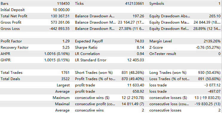
Normally for a consistently profitable EA, its backtest result should look similar to an exponential function like this:

Here are a few things to be aware of when analyzing backtest statistics when using this leverage trading model:

• If your Expert Advisor is consistently profitable, recent results will have a greater impact on the overall backtest performance than earlier ones. Essentially, you are assigning more weights to the importance of recent performance.
• LR-Correlation is not useful because the graph will be exponential curve.
• The Sharpe ratio becomes unrealistic because it assumes a linear relationship between risk and return. Leverage amplifies both potential returns and risks, leading to skewed risk-adjusted performance metrics.

If you still want to evaluate the above metrics, simply fix the lot size and do another test.

Monte Carlo Simulation of Maximum Drawdown

We view an equity curve as a series of percentage changes to our account balance, and the maximum drawdown can be seen as the segment of that series with the smallest cumulative percentage. A single backtest represents only one possible arrangement of this series, making its statistical robustness limited. The goal of this section is to understand the potential drawdowns we might encounter and to select the 95th percentile as our reference for maximum tolerance.

Monte Carlo simulation can be used to simulate a possible equity curve in several ways:

1. Random Sampling of Returns: By generating random returns based on historical performance or assumed statistical distributions (e.g., normal), you simulate potential equity curves by compounding the returns over time.

2. Bootstrapping: Resampling historical returns with replacement to create multiple simulated equity paths, which reflect the variability observed in past performance.

3. Shuffling: Randomly shuffling the order of historical returns and using the reshuffled series to generate different equity paths, allowing for a diverse set of scenarios.

4. Risk/Return Adjustments: Modifying the input parameters (e.g., volatility or drawdown limits) based on specified risk criteria to generate realistic equity curves under different market conditions.

In this article, we're going to focus on the shuffling method.

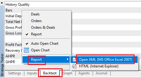
Firstly, we get the deal report from the backtest by right-clicking like this.

Then we open python and extract the useful rows that have account balance and profit/loss from each trade with this code.

import pandas as pd
# Replace 'your_file.xlsx' with the path to your file
input_file = 'DBG-XAU.xlsx'
# Load the Excel file and skip the first {skiprows} rows
data = pd.read_excel(input_file, skiprows=10757)

# Select the 'profit' column (assumed to be 'Unnamed: 10') and filter rows as per your instructions
profit_data = data[['Profit','Balance']][1:-1] 
profit_data = profit_data[profit_data.index % 2 == 0]  # Filter for rows with odd indices
profit_data = profit_data.reset_index(drop=True)  # Reset index
# Convert to float, then apply the condition to set values to 1 if > 0, otherwise to 0
profit_data = profit_data.apply(pd.to_numeric, errors='coerce').fillna(0)  # Convert to float, replacing NaN with 0
# Save the processed data to a new CSV file with index
output_csv_path = 'processed-DBG-XAU.csv'
profit_data.to_csv(output_csv_path, index=True, header=['profit_loss','account_balance'])
print(f"Processed data saved to {output_csv_path}")

The rows to skip are basically the rows above this index -1.

Next, we need to convert the profit into percentage change for each trade to ensure that the reshuffled series results in the same final balance. This is done by shifting the account balance column by one row and calculating the profit or loss as a percentage of the balance before each trade.

initial_balance = account_balance.iloc[0] - profit_loss.iloc[0]

# Calculate the account balance before each trade
account_balance_before_trade = account_balance.shift(1)
account_balance_before_trade.iloc[0] = initial_balance

# Compute the percentage change made to the account balance for each trade
percentage_change = profit_loss / account_balance_before_trade

# Fill any NaN values that might have occurred
percentage_change.fillna(0, inplace=True)

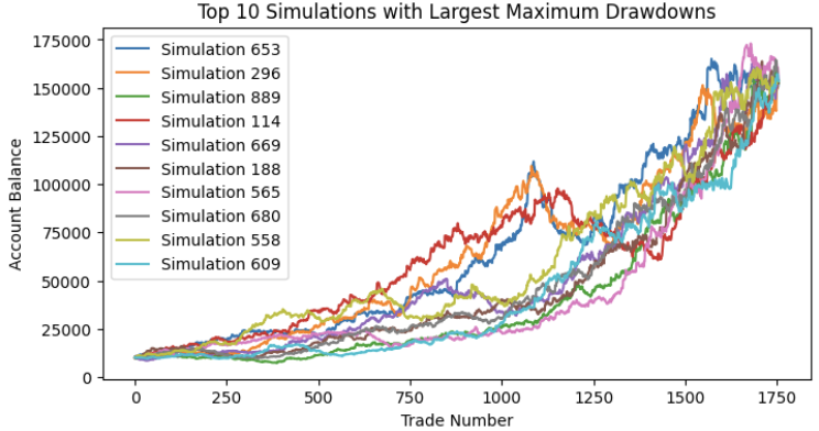
Finally, we simulate 1000 random series and plot out the top 10 with most max drawdown. Note that the final equity should all end up the same because of the Commutative Property of Multiplication. Multiplying the percentage change series will yield the same result, regardless of the order in which the values are reshuffled.

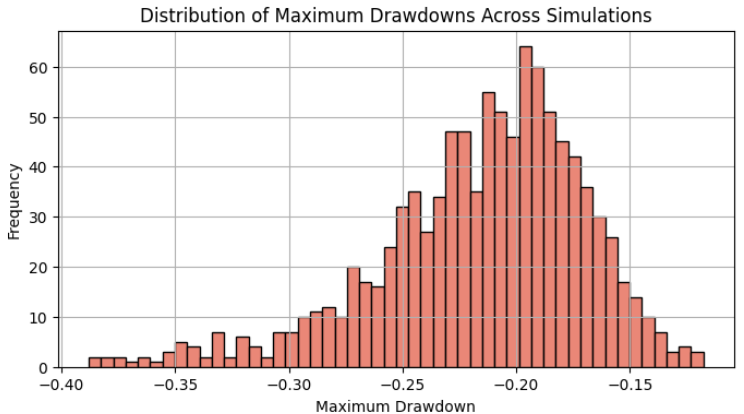
The distribution of maximum drawdown should be similar to normal distribution, and we can see here the 95% percentile (around two standard deviations) here is approximately 30% maximum drawdown.

Our initial backtest's maximum drawdown was merely 17%, which is smaller than the mean of this distribution. Had we taken it as the maximum drawdown we expected, we would have increased our risk by a factor of 2 compared to the risk we are now willing to take after obtaining the Monte Carlo simulation results. We choose the 95% percentile because it's a general result scholars see as close to live trading performance. We got lucky here that the 95% percentile aligns closely with our maximum tolerance of 30%, which was set at the beginning. This means that if we are trading this single EA in our portfolio, a 2% risk per trade will maximize our profit while keeping us well within our maximum tolerance. If the result differs, we should repeat the above procedure until we find the optimal solution.

Kelly Criterion for Portfolio Optimization

If we are running multiple EAs on a single account, we first need to complete the procedure above for each EA to determine its optimal risk. Then, we apply this risk to the allocated capital for each EA within the overall portfolio. From the perspective of the entire account, the risk amount for each EA will be the original risk multiplied by the allocated fraction.

The Kelly allocation fraction for each EA is determined by its return correlations with other EAs and its overall backtest performance. Our primary objective is to ensure that the EAs offset each other's drawdown as much as possible, resulting in a smoother equity curve for the entire portfolio. It’s important to note that adding more EAs and strategies only enhances portfolio diversity if they are uncorrelated; otherwise, it may increase the overall risk, akin to amplifying the risk of a single EA.

Specifically, we calculate the Kelly allocation fraction for each strategy based on the expected returns and the covariance matrix of returns using the following formulas:

• r: the return of EAi or EAj at time t
• μ: the mean return of EAi or EAj
  
• f: Kelly allocation for each EA
• Σ−1: the inverse of covariance matrix
  
• u: the vector of expected return for each EA

To extract the values for the variables mentioned above, we must conduct a backtest for each strategy and store the percentage return series of each strategy in a single data frame. Next, based on the frequency of all EAs, we select the appropriate time interval for recording, as the covariance is calculated based on the correlations of returns within the same time period. We perform such operations with this python code:

# Read returns for each strategy
    for file in strategy_files:
        try:
            data = pd.read_csv(file, index_col='Time')
            # Ensure 'Time' is parsed correctly as datetime
            data.index = pd.to_datetime(data.index, errors='coerce')
            
            # Drop rows where 'Time' or 'return' is invalid
            data.dropna(subset=['return'], inplace=True)
            
            # Aggregate duplicate time indices by mean (or could use 'sum', but here mean can ignore the trade frequency significance)
            data = data.groupby(data.index).agg({'return': 'mean'})
            
            # Append results
            returns_list.append(data['return'])
            strategy_names.append(file)
        except Exception as e:
            print(f"Error processing {file}: {e}")
            continue 
    # Check if any data was successfully loaded
    if not returns_list:
        print("No valid data found in files.")
        return  
    # Combine returns into a single DataFrame, aligning by date
    returns_df = pd.concat(returns_list, axis=1, keys=strategy_names) 
    # Uncomment the below line if u wanna drop rows with missing values across strategies
    #returns_df.dropna(inplace=True)
    #Uncomment the below line if u wanna just fill unaligned rows with 0( I think this is best for backtest that may have years differences)
    returns_df.fillna(0, inplace=True)

Ensure that all backtest results start and end at the same time. Additionally, select an appropriate time interval for aggregating the results so that no interval has an excessive number of trades, nor any interval with no trades at all. If the time intervals are too discrete, there may be insufficient data points within the same time ranges to calculate the covariance accurately. In our case, we select a one-month interval and use the average return for each month as the return feature.

Now we do the calculations:

    # Calculate expected returns (mean returns)
    expected_returns = returns_df.mean()
    
    # Calculate the covariance matrix of returns
    cov_matrix = returns_df.cov()
    
    # Compute the inverse of the covariance matrix
    try:
        inv_cov_matrix = np.linalg.inv(cov_matrix.values)
    except np.linalg.LinAlgError:
        # Use pseudo-inverse if covariance matrix is singular
        inv_cov_matrix = np.linalg.pinv(cov_matrix.values)
    
    # Calculate Kelly optimal fractions
    kelly_fractions = inv_cov_matrix @ expected_returns.values
    kelly_fractions = kelly_fractions / np.sum(kelly_fractions)

In the end, it will output something like this:

         Strategy  Kelly Fraction
0  A1-DBG-XAU.csv        0.211095
1   A1-DBG-SP.csv        0.682924
2   A1-DBG-EU.csv        0.105981

We can directly implement this risk into our original MQL5 code because the initial risk calculation was already based on the total account balance. As the account balance changes, the allocated capital will be automatically recalculated and applied to the next trade.

double riskAmount = AccountInfoDouble(ACCOUNT_BALANCE) * risk / 100;

For example, to apply the calculated Kelly Fraction to our example EA, we simply modify this part of the original code, and the task is completed.

input double risk = 2.0*0.211095;

I am fully aware that we could alternatively recalculate the risk based on the change in allocated capital for each EA, but basing the calculation on the entire portfolio is preferred for the following reasons:

1. Keeping track of change in different allocated capitals is intractable in my opinion. One may have to open multiple accounts or write a program to update changes after each trade.
2. The Kelly Criterion is used to maximize the long-term growth of the entire portfolio. The performance of individual EAs affects the risk of the other EAs, thereby facilitating the efficient growth of a small portfolio as it scales up.
3. If we base the risk on the change in allocated capital for each EA, the well-performing EAs will see an increase in their allocated capital over time, leading to greater risk exposure for these EAs. This undermines our initial intention of calculating risk allocation based on correlations.

However, our approach does possess certain limitations:

1. The risk for each EA fluctuates with the overall portfolio performance, making it difficult to track the performance of individual EAs. The entire portfolio can be viewed as an index like the S&P 500. To assess individual performance, one would need to calculate the percentage change rather than the absolute profit.
2. Our risk allocation calculation does not account for the trade frequency of each EA. This means that if the EAs on the same account have significantly different trade frequencies, it could lead to uneven risk exposure, despite the allocation.

Overall, considering the potential for maximizing growth for individual traders, this approach is worth adopting.

Conclusion

In this article, we introduced the Kelly Criterion within the context of the Leverage Space Trading Model and its application to trading. We then provided the implementation code in MQL5. Following this, we used Monte Carlo simulation to determine the optimal maximum drawdown to consider based on a single backtest, which was then applied to assess the risk for individual EAs. Finally, we presented an approach for capital allocation to each EA based on their backtest performance and correlations.

File Table

Name	Usage
KellyMultiFactors.ipynb	Calculate the Kelly Fractions for allocating capital
MonteCarloDrawdown.ipynb	Perform Monte Carlo Simulations