データサイエンスとML（第31回）：取引のためのCatBoost AIモデルの使用

MetaTrader 5 — トレーディング | 7 1月 2025, 08:58

173

Omega J Msigwa

「CatBoostは勾配ブースティングライブラリであり、効率的でスケーラブルな方法でカテゴリ特徴量を扱うことで差別化を図り、多くの実世界の問題に対して大幅な性能向上を提供します。」

— Anthony Goldbloom

CatBoostとは？

CatBoostは、決定木に基づく勾配ブースティングアルゴリズムを備えたオープンソースのソフトウェアライブラリであり、機械学習におけるカテゴリ特徴量やデータ処理の課題を解決するために特化して設計されています。

CatBoostはYandexによって開発され、2017年にオープンソースとして公開されました（詳細）。

CatBoostは、線形回帰やSVMなどの従来の機械学習手法と比べて比較的新しい技術であるにもかかわらず、AIコミュニティで急速に注目を集め、Kaggleのようなプラットフォームで最も利用される機械学習モデルの1つとなっています。

CatBoostが特に評価されているのは、多くの機械学習アルゴリズムが苦手とするカテゴリ特徴量の自動処理能力にあります。

このモデルは、設定やチューニングにほとんど手を加えなくても、他のモデルと比較して優れたパフォーマンスを発揮することが多いです。デフォルトのパラメータを使用した場合でも高い精度を実現できる点が大きな特長です。
また、ニューラルネットワークのように専門知識や複雑なコーディングが必要とされることがなく、CatBoostは簡単に実装できます。

この記事では、機械学習、決定木、XGBoost、LightGBM、ONNXについての基本的な理解があることを前提としています。

CatBoostの動作方法

CatBoostは、Light Gradient Machine (LightGBM)やExtreme Gradient Boosting (XGBoost)と同様に、勾配ブースティングアルゴリズムに基づいて動作します。このアルゴリズムでは、複数の決定木モデルを順次構築し、各モデルが前のモデルの誤差を補正するように設計されています。各モデルは前のモデルを土台として積み上げる形で学習を進めます。

最終的な予測は、この過程で構築されたすべてのモデルの予測を重み付きで合計することで得られます。

これらの勾配ブースティング決定木(GBDT: Gradient Boosted Decision Tree)の主な目的は、損失関数を最小化することにあります。これは、前のモデルの誤差を修正する新しいモデルを順次追加していくことで実現されます。

カテゴリ特徴量の処理

前述の通り、CatBoostは、ワンホット(One-hot)エンコーディングやラベルエンコーディングのような明示的なエンコーディングを必要とせずに、カテゴリ特徴量を直接扱うことができます。これは、CatBoostがカテゴリ特徴量に対してターゲットベースのエンコーディングを採用しているためです。

このターゲットベースのエンコーディングでは、各カテゴリ特徴値に対するターゲットの条件付き分布を計算してエンコードをおこないます。

さらに、CatBoostが革新的である点の1つに、カテゴリ特徴量の統計量を計算する際に順序付きブースティング(ordered boosting)を用いることが挙げられます。この手法により、各データポイントのエンコーディングが、以前に観測されたデータポイントの情報に基づいて計算されることが保証されます。

これにより、データ漏洩を防ぐと同時に、過剰適合のリスクを低減することが可能になります。

対称決定木構造の採用

LightGBMやXGBoostが非対称な決定木を使用しているのに対し、CatBoostは意思決定プロセスで対称決定木を採用しています。対称木では、各分岐の左枝と右枝が同じ分割ルールに基づいて対称的に構築されるのが特徴です。このアプローチには以下の利点があります。

左右対称の分割なので、訓練するのが速い
より簡単なツリー構造による効率的なメモリ使用
対称木はデータの小さな摂動に対してより頑健

CatBoostとXGBoostおよびLightGBMの詳細比較

CatBoostと他の勾配ブースト決定木との違いを理解しましょう。この3つの違いを理解することで、3つのうちのどれを使うべきで、いつ使うべきでないかを知ることができます。

側面	CatBoost	LightGBM	XGBoost
カテゴリ特徴量の取り扱い	カテゴリ変数を扱うための自動エンコードと順序付きブースティングを装備	ワンホットエンコーディング、ラベルエンコーディングなどの手動エンコーディング処理が必要	ワンホットエンコーディング、ラベルエンコーディングなどの手動エンコーディング処理が必要
決定木構造	左右対称の決定木があり、バランスよく均等に成長。予測速度が速くなり、過剰適合のリスクも低くなる。	最も損失の大きい葉に焦点を当てる葉ごとの成長戦略（非対称）を持つ。その結果、精度は高くなるが、過剰適合のリスクが高くなる。	各ノードに最適な分割に基づいてツリーを成長させるレベル単位の成長戦略（非対称）を持つ。このため、予測は柔軟だが遅くなり、過剰適合の危険性がある。
モデル精度	順序付きブースティングにより、多くのカテゴリ特徴量を含むデータセットを扱う際に優れた精度を提供し、小規模データにおける過剰適合のリスクを低減。	リーフワイズ成長戦略は、誤差の大きい領域での性能向上に重点を置いているため、特に大規模で高次元のデータセットにおいて優れた精度を提供。	ほとんどのデータセットで良好な精度を提供するが、カテゴリデータセットではCatBoostに、非常に大規模なデータセットではLightGBMに劣る傾向がある。
訓練のスピードと正確さ	通常、LightGBMよりも訓練に時間がかかるが、小～中程度のデータセットでは、特にカテゴリ特徴量が含まれる場合に効率的。	通常、最も高速であり、特に大規模なデータセットでは、高次元データでより効率的なリーフ単位のツリー成長をおこなう。	ほんのわずかな差で最も遅いことが多い。大規模なデータセットに対して非常に効率的。

CatBoostモデルの展開

CatBoostのコードを書く前に、問題のシナリオを作ってみましょう。始値、高値、安値、終値と、日（現在の日付）、曜日（月曜から日曜まで）、年（1から365まで）、月（1月から12月まで）のようないくつかのカテゴリ特徴量を使って、売買シグナル（買い/売り）を予測したいとします。

OHLC（Open、High、Low、Close）値は連続的特徴であり、その他はカテゴリ特徴量です。このデータを収集するスクリプトは添付ファイルにあります。

CatBoostモデルをインストールした後、インポートすることから始めます。

インストール

コマンドライン

pip install catboost

インポートします。

Pythonコード

import numpy as np
import pandas as pd
import catboost
from catboost import CatBoostClassifier
from sklearn.pipeline import Pipeline 
from sklearn.model_selection import train_test_split
from sklearn.metrics import classification_report
import seaborn as sns
import matplotlib.pyplot as plt

sns.set_style("darkgrid")

データを視覚化することで、それが何なのかを確認することができます。

df = pd.read_csv("/kaggle/input/ohlc-eurusd/EURUSD.OHLC.PERIOD_D1.csv")

df.head()

結果

	Open	High	Low	Close	Day	DayofWeek	DayofYear	Month
0	1.09381	1.09548	1.09003	1.09373	21.0	3.0	264.0	9.0
1	1.09678	1.09810	1.09361	1.09399	22.0	4.0	265.0	9.0
2	1.09701	1.09973	1.09606	1.09805	23.0	5.0	266.0	9.0
3	1.09639	1.09869	1.09542	1.09742	26.0	1.0	269.0	9.0
4	1.10302	1.10396	1.09513	1.09757	27.0	2.0	270.0	9.0

MQL5スクリプト内でデータを収集しているときに、DayofWeek（月曜日から日曜日）とMonth（1月から12月）の値を文字列ではなく整数として取得しました。これは、これらの値を、現状ではカテゴリ変数であるにもかかわらず、文字列を追加できないマトリックスに格納していたためです。これらの値を再びカテゴリに変換し、CatBoostでどのように処理できるかを確認します。

ターゲットとなる変数を用意しましょう。

Pythonコード

new_df = df.copy()  # Create a copy of the original DataFrame

# we Shift the 'Close' and 'open' columns by one row to ge the future close and open price values, then we add these new columns to the dataset

new_df["target_close"] = df["Close"].shift(-1)  
new_df["target_open"] = df["Open"].shift(-1)  

new_df = new_df.dropna()  # Drop the rows with NaN values resulting from the shift operation

open_values = new_df["target_open"]
close_values = new_df["target_close"]  

target = []
for i in range(len(open_values)):
    if close_values[i] > open_values[i]: 
        target.append(1) # buy signal 
    else:
        target.append(0) # sell signal

new_df["signal"] = target # we create the signal column and add the target variable we just prepared


print(new_df.shape)
new_df.head()

結果

	Open	High	Low	Close	Day	DayofWeek	DayofYear	Month	target_close	target_open	signal
0	1.09381	1.09548	1.09003	1.09373	21.0	3.0	264.0	9.0	1.09399	1.09678	0
1	1.09678	1.09810	1.09361	1.09399	22.0	4.0	265.0	9.0	1.09805	1.09701	1
2	1.09701	1.09973	1.09606	1.09805	23.0	5.0	266.0	9.0	1.09742	1.09639	1
3	1.09639	1.09869	1.09542	1.09742	26.0	1.0	269.0	9.0	1.09757	1.10302	0
4	1.10302	1.10396	1.09513	1.09757	27.0	2.0	270.0	9.0	1.10297	1.10431	0

予測可能なシグナルが得られたので、データを訓練用サンプルとテスト用サンプルに分けましょう。

X = new_df.drop(columns = ["target_close", "target_open", "signal"]) # we drop future values
y = new_df["signal"] # trading signals are the target variables we wanna predict 

X_train, X_test, y_train, y_test = train_test_split(X, y, train_size=0.7, random_state=42)

データセットに存在するカテゴリ特徴量のリストを定義します。

categorical_features = ["Day","DayofWeek", "DayofYear", "Month"]

カテゴリ変数は通常文字列形式なので、このリストを使ってカテゴリ特徴量を文字列形式に変換することができます。

X_train[categorical_features] = X_train[categorical_features].astype(str)
X_test[categorical_features] = X_test[categorical_features].astype(str)

X_train.info() # we print the data types now

結果

<class 'pandas.core.frame.DataFrame'>
Index: 6999 entries, 9068 to 7270
Data columns (total 8 columns):
 #   Column     Non-Null Count  Dtype  
---  ------     --------------  -----  
 0   Open       6999 non-null   float64
 1   High       6999 non-null   float64
 2   Low        6999 non-null   float64
 3   Close      6999 non-null   float64
 4   Day        6999 non-null   object 
 5   DayofWeek  6999 non-null   object 
 6   DayofYear  6999 non-null   object 
 7   Month      6999 non-null   object 
dtypes: float64(4), object(4)
memory usage: 492.1+ KB

これで、文字列データ型であるオブジェクトデータ型を持つカテゴリ変数ができました。このデータをCatBoost以外の機械学習モデルに適用しようとすると、オブジェクトデータ型は一般的な機械学習の学習データでは使用できないため、エラーが発生します。

CatBoostモデルの訓練

CatBoostモデルの訓練を担当するfitメソッドを呼び出す前に、このモデルを動かす多くのパラメータのいくつかを理解しましょう。

パラメータ	詳細
Iterations	決定木を構築するための反復回数です。反復回数が多いほど性能は向上しますが、過剰適合のリスクもあります。
learning_rate	この係数は、各木の最終予測への配分をコントロールします。学習率を小さくすると、ツリーが収束するまでの反復回数が増えますが、より優れたモデルになることが多いです。
depth	木の最大深度です。より深い木は、データのより複雑なパターンを捉えることができますが、しばしば過剰適合につながる可能性があります。
cat_features	カテゴリ別インデックスのリストです。 CatBoostモデルはカテゴリ特徴量を検出することができるにもかかわらず、どの特徴量がカテゴリ特徴量であるかを明示的にモデルに指示することは良い習慣です。カテゴリ変数を自動的に検出する方法が失敗することがあるため、これはモデルが人間の視点からカテゴリ特徴量を理解するのに役立ちます。
l2_leaf_reg	L2正則化係数です。より大きな葉の重みにペナルティを課すことで、過剰適合を防ぐのに役立ちます。
border_count	各カテゴリ特徴量の分割数です。この数値が高いほど性能が良くなり、計算時間が長くなります。
eval_metric	訓練中に使用される評価指標です。モデルのパフォーマンスを効果的に監視するのに役立ちます。
early_stopping_rounds	検証データがモデルに提供されたとき、このラウンド数でモデルの精度の向上が見られない場合、訓練の進行は停止します。このパラメータは過剰適合を減らし、学習時間を大幅に短縮するのに役立ちます。

上記のパラメータの辞書を定義することができます。

params = dict(
    iterations=100, 
    learning_rate=0.01,
    depth=10,
    l2_leaf_reg=5,  
    bagging_temperature=1,
    border_count=64,  # Number of splits for categorical features
    eval_metric='Logloss',
    random_seed=42,  # Seed for reproducibility
    verbose=1,  # Verbosity level
    # early_stopping_rounds=10  # Early stopping for validation
)

最後に、Sklearnパイプラインの中でCatboostモデルを定義し、このメソッドに評価データとカテゴリ特徴量のリストを与えて、訓練のためにfitメソッドを呼び出すことができます。

pipe = Pipeline([
    ("catboost", CatBoostClassifier(**params))
])

# Fit the pipeline to the training data
pipe.fit(X_train, y_train, catboost__eval_set=(X_test, y_test), catboost__cat_features=categorical_features)

出力

90:     learn: 0.6880592        test: 0.6936112 best: 0.6931239 (3)     total: 523ms    remaining: 51.7ms
91:     learn: 0.6880397        test: 0.6936100 best: 0.6931239 (3)     total: 529ms    remaining: 46ms
92:     learn: 0.6880350        test: 0.6936051 best: 0.6931239 (3)     total: 532ms    remaining: 40ms
93:     learn: 0.6880280        test: 0.6936103 best: 0.6931239 (3)     total: 535ms    remaining: 34.1ms
94:     learn: 0.6879448        test: 0.6936110 best: 0.6931239 (3)     total: 541ms    remaining: 28.5ms
95:     learn: 0.6878328        test: 0.6936387 best: 0.6931239 (3)     total: 547ms    remaining: 22.8ms
96:     learn: 0.6877888        test: 0.6936473 best: 0.6931239 (3)     total: 553ms    remaining: 17.1ms
97:     learn: 0.6877408        test: 0.6936508 best: 0.6931239 (3)     total: 559ms    remaining: 11.4ms
98:     learn: 0.6876611        test: 0.6936708 best: 0.6931239 (3)     total: 565ms    remaining: 5.71ms
99:     learn: 0.6876230        test: 0.6936898 best: 0.6931239 (3)     total: 571ms    remaining: 0us

bestTest = 0.6931239281
bestIteration = 3

Shrink model to first 4 iterations.

モデルの評価

このモデルの性能を評価するために、Sklearnメトリクスを使うことができます。

# Make predicitons on training and testing sets
y_train_pred = pipe.predict(X_train)
y_test_pred = pipe.predict(X_test)

# Training set evaluation
print("Training Set Classification Report:")
print(classification_report(y_train, y_train_pred))

# Testing set evaluation
print("\nTesting Set Classification Report:")
print(classification_report(y_test, y_test_pred))

出力

Training Set Classification Report:
              precision    recall  f1-score   support

           0       0.55      0.44      0.49      3483
           1       0.54      0.64      0.58      3516

    accuracy                           0.54      6999
   macro avg       0.54      0.54      0.54      6999
weighted avg       0.54      0.54      0.54      6999


Testing Set Classification Report:
              precision    recall  f1-score   support

           0       0.53      0.41      0.46      1547
           1       0.49      0.61      0.54      1453

    accuracy                           0.51      3000
   macro avg       0.51      0.51      0.50      3000
weighted avg       0.51      0.51      0.50      3000

結果は、平均的なパフォーマンスのモデルです。カテゴリ特徴量リストを削除した後、モデルの精度は訓練セットで60%に上昇したが、テストセットでは変わりませんでした。

pipe.fit(X_train, y_train, catboost__eval_set=(X_test, y_test))

結果

91:     learn: 0.6844878        test: 0.6933503 best: 0.6930500 (30)    total: 395ms    remaining: 34.3ms
92:     learn: 0.6844035        test: 0.6933539 best: 0.6930500 (30)    total: 399ms    remaining: 30ms
93:     learn: 0.6843241        test: 0.6933791 best: 0.6930500 (30)    total: 404ms    remaining: 25.8ms
94:     learn: 0.6842277        test: 0.6933732 best: 0.6930500 (30)    total: 408ms    remaining: 21.5ms
95:     learn: 0.6841427        test: 0.6933758 best: 0.6930500 (30)    total: 412ms    remaining: 17.2ms
96:     learn: 0.6840422        test: 0.6933796 best: 0.6930500 (30)    total: 416ms    remaining: 12.9ms
97:     learn: 0.6839896        test: 0.6933825 best: 0.6930500 (30)    total: 420ms    remaining: 8.58ms
98:     learn: 0.6839040        test: 0.6934062 best: 0.6930500 (30)    total: 425ms    remaining: 4.29ms
99:     learn: 0.6838397        test: 0.6934259 best: 0.6930500 (30)    total: 429ms    remaining: 0us

bestTest = 0.6930499562
bestIteration = 30

Shrink model to first 31 iterations.

Training Set Classification Report:
              precision    recall  f1-score   support

           0       0.61      0.53      0.57      3483
           1       0.59      0.67      0.63      3516

    accuracy                           0.60      6999
   macro avg       0.60      0.60      0.60      6999
weighted avg       0.60      0.60      0.60      6999

このモデルをさらに詳しく理解するために、特徴量の重要度プロットを作成してみましょう。

# Extract the trained CatBoostClassifier from the pipeline
catboost_model = pipe.named_steps['catboost']

# Get feature importances
feature_importances = catboost_model.get_feature_importance()

feature_im_df = pd.DataFrame({
    "feature": X.columns,
    "importance": feature_importances
})

feature_im_df = feature_im_df.sort_values(by="importance", ascending=False)

plt.figure(figsize=(10, 6))
sns.barplot(data = feature_im_df, x='importance', y='feature', palette="viridis")

plt.title("CatBoost feature importance")
plt.xlabel("Importance")
plt.ylabel("feature")
plt.show()

出力

上記の「特徴量重要度プロット」は、モデルがどのように意思決定をしていたかをすべて物語っています。CatBoostモデルは、連続変数よりもカテゴリ変数を、モデルの最終予測結果に最も影響する特徴として考慮したようです。

CatBoostモデルをONNXに保存する

このモデルをMetaTrader 5で使用するには、ONNX形式に保存する必要があります。CatBoostモデルの保存は、SklearnやKerasのモデルとは異なり、少し厄介です。

ドキュメントの指示に従った後、保存することができました。コードのほとんどは理解しようとしませんでした。

from onnx.helper import get_attribute_value
import onnxruntime as rt
from skl2onnx import convert_sklearn, update_registered_converter
from skl2onnx.common.shape_calculator import (
    calculate_linear_classifier_output_shapes,
)  # noqa
from skl2onnx.common.data_types import (
    FloatTensorType,
    Int64TensorType,
    guess_tensor_type,
)
from skl2onnx._parse import _apply_zipmap, _get_sklearn_operator_name
from catboost import CatBoostClassifier
from catboost.utils import convert_to_onnx_object

def skl2onnx_parser_castboost_classifier(scope, model, inputs, custom_parsers=None):
    
    options = scope.get_options(model, dict(zipmap=True))
    no_zipmap = isinstance(options["zipmap"], bool) and not options["zipmap"]

    alias = _get_sklearn_operator_name(type(model))
    this_operator = scope.declare_local_operator(alias, model)
    this_operator.inputs = inputs

    label_variable = scope.declare_local_variable("label", Int64TensorType())
    prob_dtype = guess_tensor_type(inputs[0].type)
    probability_tensor_variable = scope.declare_local_variable(
        "probabilities", prob_dtype
    )
    this_operator.outputs.append(label_variable)
    this_operator.outputs.append(probability_tensor_variable)
    probability_tensor = this_operator.outputs

    if no_zipmap:
        return probability_tensor

    return _apply_zipmap(
        options["zipmap"], scope, model, inputs[0].type, probability_tensor
    )


def skl2onnx_convert_catboost(scope, operator, container):
    """
    CatBoost returns an ONNX graph with a single node.
    This function adds it to the main graph.
    """
    onx = convert_to_onnx_object(operator.raw_operator)
    opsets = {d.domain: d.version for d in onx.opset_import}
    if "" in opsets and opsets[""] >= container.target_opset:
        raise RuntimeError("CatBoost uses an opset more recent than the target one.")
    if len(onx.graph.initializer) > 0 or len(onx.graph.sparse_initializer) > 0:
        raise NotImplementedError(
            "CatBoost returns a model initializers. This option is not implemented yet."
        )
    if (
        len(onx.graph.node) not in (1, 2)
        or not onx.graph.node[0].op_type.startswith("TreeEnsemble")
        or (len(onx.graph.node) == 2 and onx.graph.node[1].op_type != "ZipMap")
    ):
        types = ", ".join(map(lambda n: n.op_type, onx.graph.node))
        raise NotImplementedError(
            f"CatBoost returns {len(onx.graph.node)} != 1 (types={types}). "
            f"This option is not implemented yet."
        )
    node = onx.graph.node[0]
    atts = {}
    for att in node.attribute:
        atts[att.name] = get_attribute_value(att)
    container.add_node(
        node.op_type,
        [operator.inputs[0].full_name],
        [operator.outputs[0].full_name, operator.outputs[1].full_name],
        op_domain=node.domain,
        op_version=opsets.get(node.domain, None),
        **atts,
    )


update_registered_converter(
    CatBoostClassifier,
    "CatBoostCatBoostClassifier",
    calculate_linear_classifier_output_shapes,
    skl2onnx_convert_catboost,
    parser=skl2onnx_parser_castboost_classifier,
    options={"nocl": [True, False], "zipmap": [True, False, "columns"]},
)

最終的にモデルを変換し拡張子「.onnx」を持つファイルに保存します。

model_onnx = convert_sklearn(
    pipe,
    "pipeline_catboost",
    [("input", FloatTensorType([None, X_train.shape[1]]))],
    target_opset={"": 12, "ai.onnx.ml": 2},
)

# And save.
with open("CatBoost.EURUSD.OHLC.D1.onnx", "wb") as f:
    f.write(model_onnx.SerializeToString())

Netronで可視化すると、モデル構造はXGBoostやLightGBMと同じに見えます。

NetronにおけるCatBoostモデル

これは単なる勾配ブースティング決定木なので、理にかなっています。両者の核心は似たような構造を持っています。

パイプラインのCatBoostモデルをカテゴリ変数付きのONNXに変換しようとすると、エラーが出て処理に失敗しました。

CatBoostError: catboost/libs/model/model_export/model_exporter.cpp:96: ONNX-ML format export does yet not support categorical features

カテゴリ変数が、MetaTrader 5で最初に収集したときと同じようにfloat64 (double)型であることを確認する必要がありました。これによりエラーが修正され、MQL5でこのモデルを操作するときに、double値またはfloat値を整数と混在させることを心配する必要がなくなります。

categorical_features = ["Day","DayofWeek", "DayofYear", "Month"]

# Remove these two lines of code operations

# X_train[categorical_features] = X_train[categorical_features].astype(str)
# X_test[categorical_features] = X_test[categorical_features].astype(str)

X_train.info() # we print the data types now

CatBoostモデルは多様な性質のデータセットで動作できるため、この変更にもかかわらず、CatBoostモデルは影響を受けませんでした（同じ精度値を提供した）。

CatBoostエキスパートアドバイザー（取引ロボット）の作成

まず、ONNXモデルをリソースとしてメインのエキスパートアドバイザー(EA)に組み込みます。

MQL5コード

#resource "\\Files\\CatBoost.EURUSD.OHLC.D1.onnx" as uchar catboost_onnx[]

CatBoostモデルをロードするためのライブラリをインポートします。

#include <MALE5\Gradient Boosted Decision Trees(GBDTs)\CatBoost\CatBoost.mqh>
CCatBoost cat_boost;

OnTick関数内で訓練データを収集したのと同じ方法でデータを収集しなければなりません。

void OnTick()
 {
...
...
...     

   if (CopyRates(Symbol(), timeframe, 1, 1, rates) < 0) //Copy information from the previous bar
    {
      printf("Failed to obtain OHLC price values error = ",GetLastError());
      return;
    }
   
   MqlDateTime time_struct;
   string time = (string)datetime(rates[0].time); //converting the date from seconds to datetime then to string
   TimeToStruct((datetime)StringToTime(time), time_struct); //converting the time in string format to date then assigning it to a structure
      
   vector x = {rates[0].open,
               rates[0].high, 
               rates[0].low, 
               rates[0].close, 
               time_struct.day, 
               time_struct.day_of_week, 
               time_struct.day_of_year, 
               time_struct.mon}; //input features from the previously closed bar
...
...
...     
  }

そして最終的に、予測シグナルと、弱気シグナルクラス0と強気シグナルクラス1の間の確率ベクトルを得ることができます。

   vector proba = cat_boost.predict_proba(x); //predict the probability between the classes
   long signal = cat_boost.predict_bin(x); //predict the trading signal class
   
   Comment("Predicted Probability = ", proba,"\nSignal = ",signal);

モデルから得られた予測に基づいて取引戦略をコーディングすることで、このEAをまとめることができます。

戦略は単純で、モデルが強気シグナルを予測したら買い、売りシグナルがあったら決済します。モデルが弱気シグナルを予測した場合は、その逆をおこないます。

void OnTick()
  {
//---
   
   if (!NewBar())
    return;
   
//--- Trade at the opening of each bar

   if (CopyRates(Symbol(), timeframe, 1, 1, rates) < 0) //Copy information from the previous bar
    {
      printf("Failed to obtain OHLC price values error = ",GetLastError());
      return;
    }
   
   MqlDateTime time_struct;
   string time = (string)datetime(rates[0].time); //converting the date from seconds to datetime then to string
   TimeToStruct((datetime)StringToTime(time), time_struct); //converting the time in string format to date then assigning it to a structure
      
   vector x = {rates[0].open,
               rates[0].high, 
               rates[0].low, 
               rates[0].close, 
               time_struct.day, 
               time_struct.day_of_week, 
               time_struct.day_of_year, 
               time_struct.mon}; //input features from the previously closed bar
               
   vector proba = cat_boost.predict_proba(x); //predict the probability between the classes
   long signal = cat_boost.predict_bin(x); //predict the trading signal class
   
   Comment("Predicted Probability = ", proba,"\nSignal = ",signal);
   
//---
      
      MqlTick ticks;
      SymbolInfoTick(Symbol(), ticks);
      
      if (signal==1) //if the signal is bullish
       {
          if (!PosExists(POSITION_TYPE_BUY)) //There are no buy positions
            m_trade.Buy(min_lot, Symbol(), ticks.ask, 0, 0); //Open a buy trade
          
          ClosePosition(POSITION_TYPE_SELL); //close the opposite trade  
       }
      else //Bearish signal
        {
          if (!PosExists(POSITION_TYPE_SELL)) //There are no Sell positions
            m_trade.Sell(min_lot, Symbol(), ticks.bid, 0, 0); //open a sell trade
            
            
          ClosePosition(POSITION_TYPE_BUY); //close the opposite trade
        }
  }

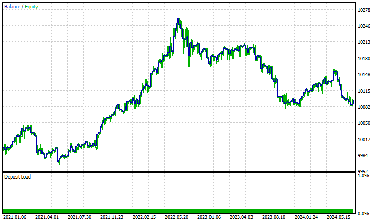
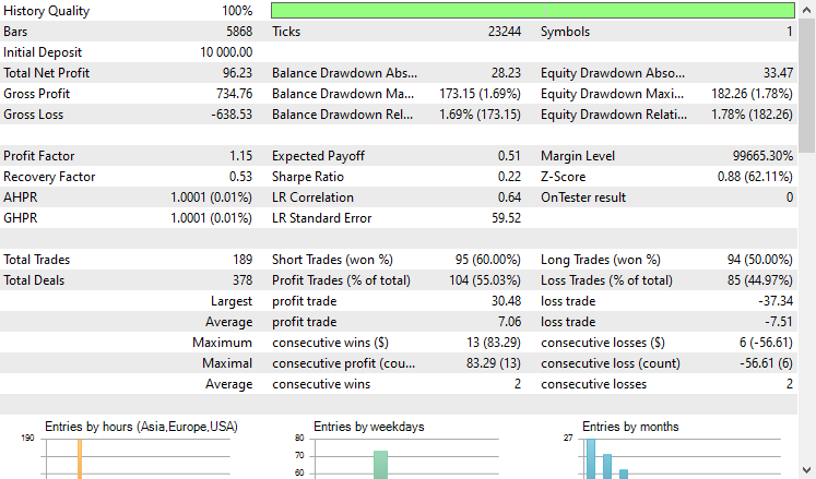
ストラテジーテスターで2021.01.01から2024.10.8まで4時間足でテストしてみました。モデルは「始値のみ」に設定されました。以下はその結果です。

EAは控えめに言ってもうまくいき、55%の利益を上げ、合計96米ドルの純利益をもたらしました。シンプルなデータセット、シンプルなモデル、最小限の取引量の設定にしては悪くありません。

最後に

CatBoostや他の勾配ブースティング決定木アルゴリズムは、限られたリソース環境で作業する際や、多数の機械学習モデルを扱う場面で、複雑な特徴エンジニアリングやモデル構成に時間を費やすことなく「そのまま機能する」モデルを求める場合に最適なソリューションです。

そのシンプルさと低い参入障壁にもかかわらず、CatBoostは多くの実世界のアプリケーションで採用されており、最も優れた、そして効果的なAIモデルの1つとして広く評価されています。

ご精読ありがとうございました。

機械学習モデルの開発を追跡し、本連載で説明されている多くのことは、このGitHubレポに掲載されています。

添付ファイルの表

ファイル名	ファイルタイプ	説明と使用法
Experts\CatBoost EA.mq5	エキスパートアドバイザー(EA)	CatboostモデルをONNX形式で読み込み、MetaTrader 5で取引戦略をテストするための自動売買ロボット
Include\CatBoost.mqh	インクルードファイル	CatBoostモデルをロードしてデプロイするためのコード
Files\ CatBoost.EURUSD.OHLC.D1.onnx	ONNXモデル	ONNX形式で保存された学習済みCatBoostモデル
Scripts\CollectData.mq5	MQL5スクリプト	訓練データを収集するスクリプト
Jupyter Notebook\CatBoost-4-trading.ipynb	Python/Jupyterノートブック	この記事で説明したすべてのPythonコードを含むノートブック

情報源と参考文献

MetaQuotes Ltdにより英語から翻訳されました。
元の記事: https://www.mql5.com/en/articles/16017

添付されたファイル |

ZIPをダウンロード

Attachments.zip (40.07 KB)

警告: これらの資料についてのすべての権利はMetaQuotes Ltd.が保有しています。これらの資料の全部または一部の複製や再プリントは禁じられています。

この著者による他の記事

ディスカッションに移動

Connexusの本体（第4回）：HTTP本体サポートの追加

この記事では、JSONやプレーンテキストなどのデータを送信するために不可欠な、HTTPリクエストにおける本体（ボディ）の概念について探りました。適切なヘッダを使った正しい使い方を議論し、説明しました。また、Connexusライブラリの一部であるChttpBodyクラスを導入し、リクエストの本体の処理を簡素化しました。

PythonとMQL5でロボットを開発する（第3回）：モデルベース取引アルゴリズムの実装

PythonとMQL5で自動売買ロボットを開発する連載を続けます。この記事では、Pythonで取引アルゴリズムを作成します。

Controlsクラスを使用してインタラクティブなMQL5ダッシュボード/パネルを作成する方法（第1回）：パネルの設定

この記事では、取引操作を効率化するために設計されたMQL5のControlsクラスを使用して、インタラクティブな取引ダッシュボードを作成します。パネルには、タイトル、[Trade]、[Close]、[Information]のナビゲーションボタン、取引の実行とポジションの管理用の専用アクションボタンが表示されます。この記事を読み終える頃には、今後の記事でさらに機能強化するための基礎パネルが完成しているはずです。

ニューラルネットワークが簡単に（第95回）：Transformerモデルにおけるメモリ消費の削減

Transformerアーキテクチャに基づくモデルは高い効率を示しますが、その使用は、訓練段階と運転中の両方で高いリソースコストによって複雑になります。この記事では、このようなモデルのメモリ使用量を削減するアルゴリズムを紹介します。