Developing a robot in Python and MQL5 (Part 1): Data preprocessing

Introduction

The market is becoming increasingly complex. Today it is turning into a battle of algorithms. Over 95% of trading turnover is generated by robots. 

The next step is machine learning. These are not strong AI, but they are not simple linear algorithms either. Machine learning model is capable of making profit in difficult conditions. It is interesting to apply machine learning to create trading systems. Thanks to neural networks, the trading robot will analyze big data, find patterns and predict price movements.

We will look at the development cycle of a trading robot: data collection, processing, sample expansion, feature engineering, model selection and training, creating a trading system via Python, and monitoring trades.

Working in Python has its own advantages: speed in the field of machine learning, as well as the ability to select and generate features. Exporting models to ONNX requires exactly the same feature generation logic as in Python, which is not easy. That is why I have selected online trading via Python.

Setting the task and choosing a tool

The goal of the project is to create a profitable and sustainable machine learning model for trading in Python. Stages of work:

• Collecting data from MetaTrader 5, loading primary features.
• Data augmentation to expand the sample.  
• Marking up data with labels.
• Feature engineering: generation, clustering, selection.
• Selection and training of ML model. Possibly, ensembling.
• Evaluation of models by metrics.
• Tester development for profitability assessment.  
• Achieving a positive result based on new data.
• Implementation of a trading algorithm via Python MQL5.
• Integration with MetaTrader 5.
• Improving models.

Tools: Python MQL5, ML libraries in Python for speed and functionality.

So, we have defined the goals and objectives. We will carry out the following works within the article framework:

• Collecting data from MetaTrader 5, loading primary features.
• Data augmentation to expand the sample.  
• Marking up data with labels.
• Feature engineering: generation, clustering, selection.

Setting up the environment and imports. Data collection

First, we need to get historical data via MetaTrader 5. The code establishes a connection to the trading platform by passing the path to the terminal file to the initialization method.

In the loop, get data using the mt5.copy_rates_range() method with the following parameters: instrument, timeframe, start and end dates. There is a counter of unsuccessful attempts and a delay for a stable connection.

The function terminates by disconnecting from the platform using the mt5.shutdown() method.

This is a separate function for further calling in the program. 

To run the script, you will need to install the following libraries:

1. NumPy: The library for working with multidimensional arrays and mathematical functions.

2. Pandas: A data analysis tool that provides convenient data structures for working with tables and time series.

3. Random: Module for generating random numbers and selecting random elements from sequences.

4. Datetime: Provides classes and functions for working with dates and time.

5. MetaTrader5: Library for interaction with the MetaTrader 5 trading terminal.

6. Time: Module for working with time and program execution delays.

7. Concurrent.futures: The tool for running parallel and asynchronous tasks. We will need this in the future for parallel multi-currency work.

8. Tqdm: The library for displaying progress indicators when performing iterative operations. We will need this in the future for parallel multi-currency work.

9. Train_test_split: Function to split a dataset into training and testing sets when training machine learning models.

You can install them using 'pip' by running the following commands:

pip install numpy pandas MetaTrader5 concurrent-futures tqdm sklearn matplotlib imblearn

import numpy as np
import pandas as pd
import random
from datetime import datetime
import MetaTrader5 as mt5
import time
import concurrent.futures
from tqdm import tqdm
from sklearn.model_selection import train_test_split
import matplotlib.pyplot as plt
from sklearn.utils import class_weight
from imblearn.under_sampling import RandomUnderSampler

# GLOBALS
MARKUP = 0.00001
BACKWARD = datetime(2000, 1, 1)
FORWARD = datetime(2010, 1, 1)
EXAMWARD = datetime(2024, 1, 1)
MAX_OPEN_TRADES = 3
symbol = "EURUSD"

def retrieve_data(symbol, retries_limit=300):
    terminal_path = "C:/Program Files/MetaTrader 5/Arima/terminal64.exe"

    attempt = 0
    raw_data = None

    while attempt < retries_limit:
        if not mt5.initialize(path=terminal_path):
            print("MetaTrader initialization failed")
            return None

        instrument_count = mt5.symbols_total()
        if instrument_count > 0:
            print(f"Number of instruments in the terminal: {instrument_count}")
        else:
            print("No instruments in the terminal")

        rates = mt5.copy_rates_range(symbol, mt5.TIMEFRAME_H1, BACKWARD, EXAMWARD)
        mt5.shutdown()

        if rates is None or len(rates) == 0:
            print(f"Data for {symbol} not available (attempt {attempt+1})")
            attempt += 1
            time.sleep(1)
        else:
            raw_data = pd.DataFrame(rates[:-1], columns=['time', 'open', 'high', 'low', 'close', 'tick_volume'])
            raw_data['time'] = pd.to_datetime(raw_data['time'], unit='s')
            raw_data.set_index('time', inplace=True)
            break

    if raw_data is None:
        print(f"Data retrieval failed after {retries_limit} attempts")
        return None

    # Add simple features
    raw_data['raw_SMA_10'] = raw_data['close'].rolling(window=10).mean()
    raw_data['raw_SMA_20'] = raw_data['close'].rolling(window=20).mean()
    raw_data['Price_Change'] = raw_data['close'].pct_change() * 100

    # Additional features
    raw_data['raw_Std_Dev_Close'] = raw_data['close'].rolling(window=20).std()
    raw_data['raw_Volume_Change'] = raw_data['tick_volume'].pct_change() * 100

    raw_data['raw_Prev_Day_Price_Change'] = raw_data['close'] - raw_data['close'].shift(1)
    raw_data['raw_Prev_Week_Price_Change'] = raw_data['close'] - raw_data['close'].shift(7)
    raw_data['raw_Prev_Month_Price_Change'] = raw_data['close'] - raw_data['close'].shift(30)

    raw_data['Consecutive_Positive_Changes'] = (raw_data['Price_Change'] > 0).astype(int).groupby((raw_data['Price_Change'] > 0).astype(int).diff().ne(0).cumsum()).cumsum()
    raw_data['Consecutive_Negative_Changes'] = (raw_data['Price_Change'] < 0).astype(int).groupby((raw_data['Price_Change'] < 0).astype(int).diff().ne(0).cumsum()).cumsum()
    raw_data['Price_Density'] = raw_data['close'].rolling(window=10).apply(lambda x: len(set(x)))
    raw_data['Fractal_Analysis'] = raw_data['close'].rolling(window=10).apply(lambda x: 1 if x.idxmax() else (-1 if x.idxmin() else 0))
    raw_data['Price_Volume_Ratio'] = raw_data['close'] / raw_data['tick_volume']
    raw_data['Median_Close_7'] = raw_data['close'].rolling(window=7).median()
    raw_data['Median_Close_30'] = raw_data['close'].rolling(window=30).median()
    raw_data['Price_Volatility'] = raw_data['close'].rolling(window=20).std() / raw_data['close'].rolling(window=20).mean()

    print("\nOriginal columns:")
    print(raw_data[['close', 'high', 'low', 'open', 'tick_volume']].tail(100))

    print("\nList of features:")
    print(raw_data.columns.tolist())

    print("\nLast 100 features:")
    print(raw_data.tail(100))

    # Replace NaN values with the mean
    raw_data.fillna(raw_data.mean(), inplace=True)

    return raw_data

retrieve_data(symbol)

Define global variables: spread costs and broker commissions, dates for training and test samples, maximum number of trades, symbol.

Loading quotes from MetaTrader 5 in a loop. The data is converted into a DataFrame and enriched with features:

• 10 and 20 period SMA moving averages
• Price change 
• Standard price deviation
• Volume change
• Daily/monthly price change
• Price medians

These features help to take into account the factors that influence the price.

Information about the DataFrame columns and latest entries is displayed.

Let's see how our first function was executed:

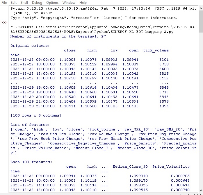
Everything works. The code successfully loaded quotes, prepared and loaded features. Let's move on to the next part of the code.

Data augmentation to expand the sample

Data augmentation is generation of new training examples based on existing ones to increase the sample size and improve the model quality. It is relevant for forecasting time series with limited data. Besides, it reduces model errors and increases robustness.

Financial data augmentation methods:

• Adding noise (random deviations) for robustness against noise
• Time shift for modeling different development scenarios
• Scaling to model price spikes/drops
• Source data inversion

I have implemented the input augmentation function that accepts DataFrame and the number of new examples for each method. It generates new data using different approaches and concatenates it with the original DataFrame.

def augment_data(raw_data, noise_level=0.01, time_shift=1, scale_range=(0.9, 1.1)):
    print(f"Number of rows before augmentation: {len(raw_data)}")

    # Copy raw_data into augmented_data
    augmented_data = raw_data.copy()

    # Add noise
    noisy_data = raw_data.copy()
    noisy_data += np.random.normal(0, noise_level, noisy_data.shape)

    # Replace NaN values with the mean
    noisy_data.fillna(noisy_data.mean(), inplace=True)

    augmented_data = pd.concat([augmented_data, noisy_data])
    print(f"Added {len(noisy_data)} rows after adding noise")

    # Time shift
    shifted_data = raw_data.copy()
    shifted_data.index += pd.DateOffset(hours=time_shift)

    # Replace NaN values with the mean
    shifted_data.fillna(shifted_data.mean(), inplace=True)

    augmented_data = pd.concat([augmented_data, shifted_data])
    print(f"Added {len(shifted_data)} rows after time shift")

    # Scaling
    scale = np.random.uniform(scale_range[0], scale_range[1])
    scaled_data = raw_data.copy()
    scaled_data *= scale

    # Replace NaN values with the mean
    scaled_data.fillna(scaled_data.mean(), inplace=True)

    augmented_data = pd.concat([augmented_data, scaled_data])
    print(f"Added {len(scaled_data)} rows after scaling")

    # Inversion
    inverted_data = raw_data.copy()
    inverted_data *= -1

    # Replace NaN values with the mean
    inverted_data.fillna(inverted_data.mean(), inplace=True)

    augmented_data = pd.concat([augmented_data, inverted_data])
    print(f"Added {len(inverted_data)} rows after inversion")

    print(f"Number of rows after augmentation: {len(augmented_data)}")

    # Print dates by years
    print("Print dates by years:")
    for year, group in augmented_data.groupby(augmented_data.index.year):
        print(f"Year {year}: {group.index}")

    return augmented_data

Call the code and get the following results:

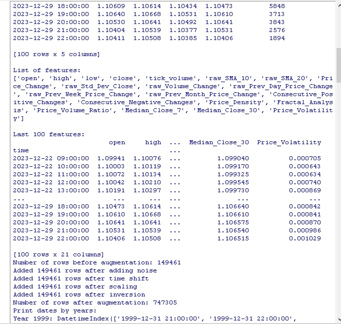
After applying data augmentation methods, our original set of 150,000 H1 price bars was expanded to an impressive 747,000 strings. Many authoritative studies in machine learning show that such a significant increase in the volume of training data due to the generation of synthetic examples has a positive effect on the quality metrics of trained models. We expect that in our case this technique will also produce the desired effect.

Label data

Data labeling is critical to the success of supervised learning algorithms. It allows us to provide the source data with labels that the model then learns. Labeled data improves accuracy, improves generalization, speeds up training and makes it easier to evaluate models. In the EURUSD forecasting problem, we added the "labels" binary column indicating whether the next price change was greater than the spread and commission. This allows the model to learn patterns of spread replay and non-rollback trends.

Labeling plays a key role allowing machine learning algorithms to find complex patterns in data that are not visible in its raw form. Let's move on to the code review.

def markup_data(data, target_column, label_column, markup_ratio=0.00002):
    data.loc[:, label_column] = np.where(data.loc[:, target_column].shift(-1) > data.loc[:, target_column] + markup_ratio, 1, 0)

    data.loc[data[label_column].isna(), label_column] = 0

    print(f"Number of markups on price change greater than markup: {data[label_column].sum()}")

    return data

Execute this code and get the number of labels in the data. The function returns a frame. Everything works. By the way, out of over 700,000 data points, the price changed by more than the spread only in 70,000 cases.

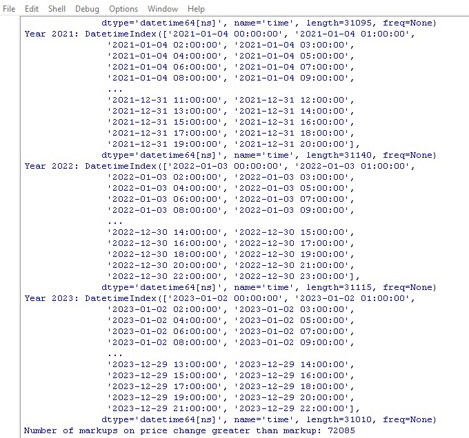
Now we have another data markup feature. This time, it is closer to actual earnings.

Target labels function

def label_data(data, symbol, min=2, max=48):
    terminal_path = "C:/Program Files/MetaTrader 5/Arima/terminal64.exe"

    if not mt5.initialize(path=terminal_path):
        print("Error connecting to MetaTrader 5 terminal")
        return

    symbol_info = mt5.symbol_info(symbol)
    stop_level = 100 * symbol_info.point
    take_level = 800 * symbol_info.point

    labels = []

    for i in range(data.shape[0] - max):
        rand = random.randint(min, max)
        curr_pr = data['close'].iloc[i]
        future_pr = data['close'].iloc[i + rand]
        min_pr = data['low'].iloc[i:i + rand].min()
        max_pr = data['high'].iloc[i:i + rand].max()

        price_change = abs(future_pr - curr_pr)

        if price_change > take_level and future_pr > curr_pr and min_pr > curr_pr - stop_level:
            labels.append(1)  # Growth
        elif price_change > take_level and future_pr < curr_pr and max_pr < curr_pr + stop_level:
            labels.append(0)  # Fall
        else:
            labels.append(None)

    data = data.iloc[:len(labels)].copy()
    data['labels'] = labels

    data.dropna(inplace=True)

    X = data.drop('labels', axis=1)
    y = data['labels']

    rus = RandomUnderSampler(random_state=2)
    X_balanced, y_balanced = rus.fit_resample(X, y)

    data_balanced = pd.concat([X_balanced, y_balanced], axis=1)

    return data

The function obtains target labels for training machine learning models on trading profits. The function connects to MetaTrader 5, retrieves symbol information and calculates stop/take levels. Then, the future price is determined after a random period for each entry point. If the price change exceeds the take profit and does not touch the stop, as well as satisfies the conditions of growth/fall, the 1.0/0.0 mark is added accordingly. Otherwise - None. A new dataframe with only the labeled data is created. None is replaced with averages.

The number of growth/fall labels is displayed.

Everything works as intended. We have received data and its derivatives. The data has been augmented, significantly supplemented and marked with two different functions. Let's move on to the next step - class balancing.

By the way, I believe that readers experienced in machine learning has long understood that we will ultimately develop a classification model, not a regression one. I like regression models better, since I see a little more predictive logic in them than in classification models. 

So, our next move is class balancing.

Balancing classes. Classification

Classification is a fundamental method of analysis based on the natural human ability to structure information according to common features. One of the first applications of classification was prospecting - identifying promising areas based on geological features.

With the advent of computers, classification has reached a new level, but the essence remains - discovering patterns in the apparent chaos of details. For financial markets, it is important to classify price dynamics into growth/fall. However, classes can be unbalanced - there are few trends and many flats.

Therefore, class balancing methods are used: removing dominant examples or generating rare ones. This allows the models to reliably recognize important but rare price dynamics patterns.

pip install imblearn

    data = data.iloc[:len(labels)].copy()
    data['labels'] = labels

    data.dropna(inplace=True)

    X = data.drop('labels', axis=1)
    y = data['labels']

    rus = RandomUnderSampler(random_state=2)
    X_balanced, y_balanced = rus.fit_resample(X, y)

    data_balanced = pd.concat([X_balanced, y_balanced], axis=1)

So, our classes are now balanced. We have an equal number of labels for each class (price drop and fall).

Let's move on to the most important thing in data forecasting - features.

What are features in machine learning?

Attributes and characteristics are basic concepts familiar to everyone from childhood. When we describe an object, we list its properties - these are the attributes. A set of such characteristics allows us to fully characterize an object.

The same thing in data analysis - each observation is described by a set of numerical and categorical features. The selection of informative features is critical to success.

At a higher level, we have feature engineering, when new derived characteristics are constructed from the initial parameters to better describe the object of study.

Thus, the human experience of knowing the world through the description of objects by their characteristics is transferred to science at the level of formalization and automation.

Automatic feature extraction

Feature engineering is the transformation of source data into a set of features for training machine learning models. The goal is to find the most informative features. There is a manual approach (a person selects features) and an automatic approach (using algorithms).

We will use the automatic approach. Let's apply the feature generation method to automatically extract the best features from our data. Then select the most informative ones from the resulting set.

Method of generating new features: 

def generate_new_features(data, num_features=200, random_seed=1):
    random.seed(random_seed)
    new_features = {}

    for _ in range(num_features):
        feature_name = f'feature_{len(new_features)}'

        col1_idx, col2_idx = random.sample(range(len(data.columns)), 2)
        col1, col2 = data.columns[col1_idx], data.columns[col2_idx]

        operation = random.choice(['add', 'subtract', 'multiply', 'divide', 'shift', 'rolling_mean', 'rolling_std', 'rolling_max', 'rolling_min', 'rolling_sum'])

        if operation == 'add':
            new_features[feature_name] = data[col1] + data[col2]
        elif operation == 'subtract':
            new_features[feature_name] = data[col1] - data[col2]
        elif operation == 'multiply':
            new_features[feature_name] = data[col1] * data[col2]
        elif operation == 'divide':
            new_features[feature_name] = data[col1] / data[col2]
        elif operation == 'shift':
            shift = random.randint(1, 10)
            new_features[feature_name] = data[col1].shift(shift)
        elif operation == 'rolling_mean':
            window = random.randint(2, 20)
            new_features[feature_name] = data[col1].rolling(window).mean()
        elif operation == 'rolling_std':
            window = random.randint(2, 20)
            new_features[feature_name] = data[col1].rolling(window).std()
        elif operation == 'rolling_max':
            window = random.randint(2, 20)
            new_features[feature_name] = data[col1].rolling(window).max()
        elif operation == 'rolling_min':
            window = random.randint(2, 20)
            new_features[feature_name] = data[col1].rolling(window).min()
        elif operation == 'rolling_sum':
            window = random.randint(2, 20)
            new_features[feature_name] = data[col1].rolling(window).sum()

    new_data = pd.concat([data, pd.DataFrame(new_features)], axis=1)

    print("\nGenerated features:")
    print(new_data[list(new_features.keys())].tail(100))

    return data

Please pay attention to the following parameter:

random_seed=42

The random_seed parameter is necessary for reproducibility of the results of generating new features. The generate_new_features function creates new features from the source data. Input: data, number of features, seed.

Random is initialized with a given seed. In the loop: a name is generated, 2 existing features and an operation (addition, subtraction, etc.) are randomly selected. A new feature for the selected operation is calculated.

After generation, new features are added to the original data. Updated data with automatically generated features is returned.

The code allows us to automatically create new features to improve the quality of machine learning.

Let's launch the code and have a look at the result:

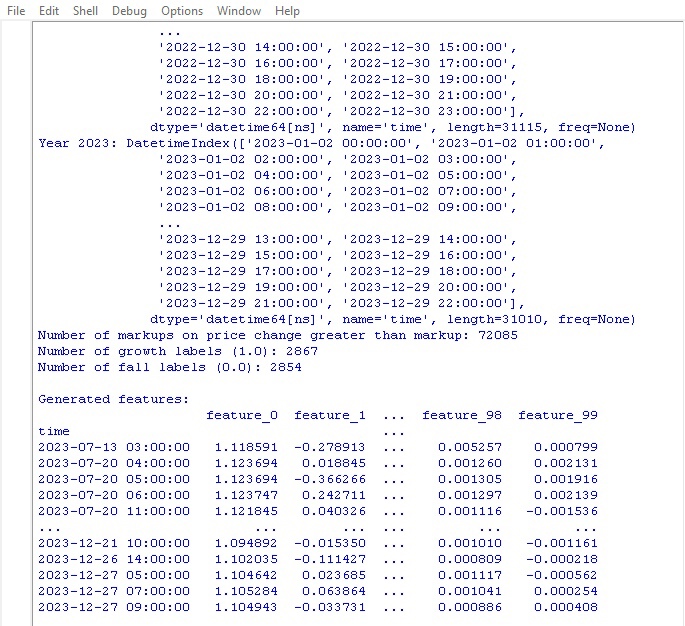
100 new features generated. Let's move on to the next stage - clustering of features.

Clustering of features

Feature clustering groups similar features into groups to reduce their number. This helps to remove redundant data, reduce correlation and simplify the model without overfitting.

Popular algorithms: k-means (the number of clusters is specified, features are grouped around centroids) and hierarchical clustering (multi-level tree structure).

Clustering of features allows us to sort out a bunch of useless features and improve the model efficiency.

Let's look at the feature clustering code:

from sklearn.mixture import GaussianMixture

def cluster_features_by_gmm(data, n_components=4):
    X = data.drop(['label', 'labels'], axis=1)

    X = X.replace([np.inf, -np.inf], np.nan)
    X = X.fillna(X.median())

    gmm = GaussianMixture(n_components=n_components, random_state=1)

    gmm.fit(X)

    data['cluster'] = gmm.predict(X)

    print("\nFeature clusters:")
    print(data[['cluster']].tail(100))

    return data

We use GMM (Gaussian Mixture Model) algorithm for feature clustering. The basic idea is that the data is generated as a mixture of normal distributions, where each distribution is one cluster.

First, set the number of clusters. Then we set the initial parameters of the model: means, covariance matrices and cluster probabilities. The algorithm cyclically recalculates these parameters using the maximum likelihood method until they stop changing.

As a result, we obtain the final parameters for each cluster, by which we can determine which cluster the new feature belongs to.

GMM is a cool thing. It is used in different tasks. It is good for data where clusters have complex shapes and blurred boundaries.

This code uses GMM to partition features into clusters. The original data is taken and class labels are removed. GMM is used to partition into a given number of clusters. Cluster numbers are added as a new column. At the end, a table of the obtained clusters is printed.

Let's run the clustering code and see the results:

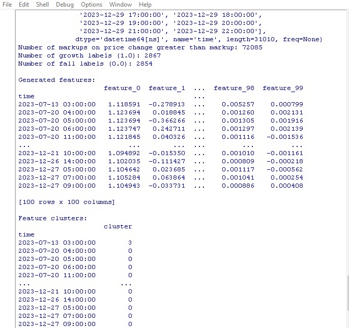
Let's move on to the function of selecting the best features.

Selecting the best features

from sklearn.feature_selection import RFECV
from sklearn.ensemble import RandomForestClassifier
import pandas as pd

def feature_engineering(data, n_features_to_select=10):
    # Remove the 'label' column as it is not a feature
    X = data.drop(['label', 'labels'], axis=1)
    y = data['labels']

    # Create a RandomForestClassifier model
    clf = RandomForestClassifier(n_estimators=100, random_state=1)

    # Use RFECV to select n_features_to_select best features
    rfecv = RFECV(estimator=clf, step=1, cv=5, scoring='accuracy', n_jobs=-1, verbose=1,
                  min_features_to_select=n_features_to_select)
    rfecv.fit(X, y)

    # Return a DataFrame with the best features, 'label' column, and 'labels' column
    selected_features = X.columns[rfecv.get_support(indices=True)]
    selected_data = data[selected_features.tolist() + ['label', 'labels']]  # Convert selected_features to a list

    # Print the table of best features
    print("\nBest features:")
    print(pd.DataFrame({'Feature': selected_features}))

    return selected_data

labeled_data_engineered = feature_engineering(labeled_data_clustered, n_features_to_select=10)

This function extracts the coolest and most useful features from our data. The input is the original data with class features and labels plus the required number of selected features.

First, class labels are reset because they will not help in feature selection. Then the Random Forest algorithm is launched - a model that builds a bunch of decision trees on random sets of features.

After training all the trees, Random Forest evaluates how important each feature is and how much it affects the classification. Based on these importance scores, the function selects the top features.

Finally, the selected features are added to the data and the class labels are returned. The function prints a table with the selected features and returns updated data.

Why all this fuss? That is how we get rid of junk features that only slow down the process. We leave the coolest features, so that the model shows better results, training on such data.

Let's launch the function and see the results:

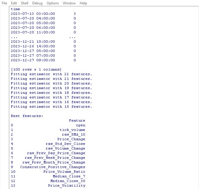
The best indicator for price forecasting turned out to be the opening price itself. The top included features based on moving averages, price increments, standard deviation, daily and monthly price changes. Automatically generated features turned out to be uninformative.

The code allows for auto selection of important features, which can improve the model performance and generalization ability.

Conclusion

We have created data manipulation code that anticipates the development of our future machine learning model. Let's briefly review the steps taken:

• The initial data for EURUSD was extracted from the MetaTrader 5 platform. Then transformations were performed using random operations - noise imposition, shifts and scaling to significantly increase the sample size.
• The next step was to mark price values with special trend markers - growth and fall, taking into account stop loss and take profit levels. To balance the classes, redundant examples were removed.
• Next, a complex feature engineering procedure was carried out. First, hundreds of new derived features were automatically generated from the original time series. Gaussian mixture clustering was then performed to detect redundancy. Finally, the random forest algorithm was used to rank and select the most informative subset of variables.
• As a result, a high-quality enriched dataset with optimal features was generated. It will serve as a basis for further training of machine learning models and development of a trading strategy in Python with integration into MetaTrader 5.

In the next article, we will focus on choosing the optimal classification model, improving it, implementing cross-validation and writing a tester function for the Python/MQL5 bundle.