Neural Network in Practice: Secant Line

Introduction

Welcome, my dear readers, to a topic that will not be treated as a series of articles.

Although many may think that it would be better to release a series of articles on the topic of artificial intelligence, I cannot imagine how this could be done. Most people have no idea about the true purpose of neural networks and, accordingly, about the so-called artificial intelligence.

So, we will not go into this topic in detail here. Instead, we will focus on other aspects. Therefore, you can read my articles on this topic in any order and focus on the material that is relevant to you. We will consider the topic of neural networks and artificial intelligence as broadly as possible. The main purpose is not to create a system oriented towards the market or some specific task. The purpose here is to explain and show how a computer program can do what has been shown in the media and what has fascinated so many people, making them believe that neural networks or artificial intelligence can have some level of consciousness.

I see a difference between neural networks and artificial intelligence, but this is, of course, just my opinion. In these articles, you will see that there is nothing special about artificial intelligence and neural networks. It is simply a well-thought-out program aimed at achieving a specific goal. However, let's not rush things just yet. First, we have to go through the different stages to understand how everything works. We will not use anything but MQL5.

This will be a personal challenge for me. I just want to show that with the right concepts and understanding of how things actually work, you can use any language to create what will be shown in this article. So, I wish you all a pleasant reading and I hope that these articles will be interesting for you and will enrich your knowledge on this topic.

Linear Regression

As already explained in the theoretical part, when working with neural networks we need to use linear regressions and derivatives. Why? The reason is that linear regression is one of the simplest formulas in existence. In fact, linear regression is just an affine function. However, when we talk about neural networks, we are not interested in the effects of direct linear regression. We are interested in the equation that generates this line. We are not interested in the line created but in the formula.

To understand this, let's create a small indicator as shown in the code below.

01. //+------------------------------------------------------------------+
02. #property copyright "Daniel Jose"
03. #property indicator_chart_window
04. #property indicator_plots 0
05. //+------------------------------------------------------------------+
06. #include <Canvas\Canvas.mqh>
07. //+------------------------------------------------------------------+
08. CCanvas canvas;
09. //+------------------------------------------------------------------+
10. void Func_01(const int x, const int y)
11. {
12.     int A[] {
13.                 -100,  150,
14.                  -80,   50,
15.                   30,  -80,
16.                  100, -120
17.             };
18. 
19.     canvas.LineVertical(x, y - 200, y + 200, ColorToARGB(clrRoyalBlue, 255));
20.     canvas.LineHorizontal(x - 200, x + 200, y, ColorToARGB(clrRoyalBlue, 255));
21. 
22.     for (uint c0 = 0, c1 = 0; c1 < A.Size(); c0++)
23.         canvas.FillCircle(x + A[c1++], y + A[c1++], 5, ColorToARGB(clrRed, 255));
24. }
25. //+------------------------------------------------------------------+
26. int OnInit()
27. {    
28.     int px, py;
29.     
30.     px = (int)ChartGetInteger(0, CHART_WIDTH_IN_PIXELS, 0);
31.     py = (int)ChartGetInteger(0, CHART_HEIGHT_IN_PIXELS, 0);
32. 
33.     canvas.CreateBitmapLabel("BL", 0, 0, px, py, COLOR_FORMAT_ARGB_NORMALIZE);
34.     canvas.Erase(ColorToARGB(clrWhite, 255));
35.         
36.     Func_01(px / 2, py / 2);
37. 
38.     canvas.Update(true);
39.     
40.     return INIT_SUCCEEDED;
41. }
42. //+------------------------------------------------------------------+
43. int OnCalculate(const int rates_total, const int prev_calculated, const int begin, const double &price[])
44. {
45.     return rates_total;
46. }
47. //+------------------------------------------------------------------+
48. void OnChartEvent(const int id, const long &lparam, const double &dparam, const string &sparam)
49. {
50. }
51. //+------------------------------------------------------------------+
52. void OnDeinit(const int reason)
53. {
54.     canvas.Destroy();
55. }
56. //+------------------------------------------------------------------+

The execution of this code generates the following on the screen.

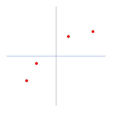
This is where we should start to understand why we would use linear regression and derivatives when working with neural networks. The red dots represent the information in the neural network, i.e., the AI has been trained and contains the information that is displayed as red dots. The blue lines are the coordinate axes. The question is, what mathematical equation best describes this data set? In other words, if we were to generalize the concepts depicted in the picture above, which mathematical formula would best represent this image? Looking at the distribution of points, you can say that it is a straight line. Then we could think about the line equation that is an affine function. This equation is shown below.

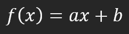
So, this function is used to create a straight line. Now let's get back to the main question. What values of A and B should we use to create the straight line in the best possible way? Well, many may say that you need to look for them by trial and error. But let's simplify things. For this, we will assume that B is equal to zero. That is, the straight line will pass through the origin of the coordinate axis. First, we will do this just for simplicity to understand the mathematics used in the neural network.

In this case, we just need to find the value of the constant A. Now another question arises: how are we going to find this value for A? You can put any, but depending on the value used, the formula will not be truly optimized. Even for such a small amount of knowledge stored in our neural network, it would not be worth losing it. For this reason, we do not (or cannot) use any meaning. We need to find the value at which A would be the best possible value.

This is where the machine begins to learn. So, this is where the term Machine Learning (ML) comes in . Many people use this term without understanding its meaning. The idea is exactly that: to create a mathematical equation that best represents the knowledge points within the network. Doing this manually is one of the most difficult tasks. However, using mathematical manipulation, we can force the machine to generate an equation for us. This is what refers to a machine learning system. The idea is to somehow get the computer to automatically generate a mathematical equation.

Now you've started to understand how a machine learns. This is just one way to do it, but there are others. However, now we will focus on this particular method. We already have a specific task that we need to accomplish. We must calculate how we can find the optimal value of the constant A in the affine equation shown above.

You could think that we can create a loop that iterates over all values in a given range. This will actually work, but it won't be computationally efficient. Think about the following: in this example, we only need one variable, the constant A. Because we consider the value of the constant B to be equal to zero. However, in practice, the constant B will most likely not be zero. Therefore, this method of traversing a range of values does not work in all situations. We need to construct something that can adapt to all situations, even if we have to change the value of the constant B.

So, how can we resolve this issue? To make things easier to understand, we'll modify this approach a little to better visualize the math that will be used. The new code is shown below:

01. //+------------------------------------------------------------------+
02. #property copyright "Daniel Jose"
03. #property indicator_chart_window
04. #property indicator_plots 0
05. //+------------------------------------------------------------------+
06. #include <Canvas\Canvas.mqh>
07. //+------------------------------------------------------------------+
08. #define _ToRadians(A) (A * (M_PI / 180.0))
09. #define _SizeLine 200
10. //+------------------------------------------------------------------+
11. CCanvas canvas;
12. //+------------------------------------------------------------------+
13. struct st_00
14. {
15.     int     x,
16.             y;
17.     double  Angle;
18. }global;
19. //+------------------------------------------------------------------+
20. void Func_01(void)
21. {
22.     int A[] {
23.                   -100,  150,
24.                    -80,   50,
25.                     30,  -80,
26.                    100, -120
27.             };
28. 
29.     canvas.LineVertical(global.x, global.y - _SizeLine, global.y + _SizeLine, ColorToARGB(clrRoyalBlue, 255));
30.     canvas.LineHorizontal(global.x - _SizeLine, global.x + _SizeLine, global.y, ColorToARGB(clrRoyalBlue, 255));
31. 
32.     for (uint c0 = 0, c1 = 0; c1 < A.Size(); c0++)
33.         canvas.FillCircle(global.x + A[c1++], global.y + A[c1++], 5, ColorToARGB(clrRed, 255));
34. }
35. //+------------------------------------------------------------------+
36. void NewAngle(const char direct, const double step = 1)
37. {
38.     canvas.Erase(ColorToARGB(clrWhite, 255));
39.     Func_01();
40. 
41.     global.Angle = (MathAbs(global.Angle + (step * direct)) <= 90 ? global.Angle + (step * direct) : global.Angle);
42.     canvas.TextOut(global.x + 250, global.y, StringFormat("%.2f", global.Angle), ColorToARGB(clrBlack));
43.     canvas.Line(
44.                 global.x - (int)(_SizeLine * cos(_ToRadians(global.Angle))), 
45.                 global.y - (int)(_SizeLine * sin(_ToRadians(global.Angle))), 
46.                 global.x + (int)(_SizeLine * cos(_ToRadians(global.Angle))), 
47.                 global.y + (int)(_SizeLine * sin(_ToRadians(global.Angle))), 
48.                 ColorToARGB(clrForestGreen)
49.             );
50.     canvas.Update(true);
51. }
52. //+------------------------------------------------------------------+
53. int OnInit()
54. {    
55.     global.Angle = 0;
56.     global.x = (int)ChartGetInteger(0, CHART_WIDTH_IN_PIXELS, 0);
57.     global.y = (int)ChartGetInteger(0, CHART_HEIGHT_IN_PIXELS, 0);
58. 
59.     canvas.CreateBitmapLabel("BL", 0, 0, global.x, global.y, COLOR_FORMAT_ARGB_NORMALIZE);
60.     global.x /= 2;
61.     global.y /= 2;
62.         
63.     NewAngle(0);
64. 
65.     canvas.Update(true);
66.     
67.     return INIT_SUCCEEDED;
68. }
69. //+------------------------------------------------------------------+
70. int OnCalculate(const int rates_total, const int prev_calculated, const int begin, const double &price[])
71. {
72.     return rates_total;
73. }
74. //+------------------------------------------------------------------+
75. void OnChartEvent(const int id, const long &lparam, const double &dparam, const string &sparam)
76. {
77.     switch (id)
78.     {
79.         case CHARTEVENT_KEYDOWN:
80.             if (TerminalInfoInteger(TERMINAL_KEYSTATE_LEFT))
81.                 NewAngle(-1);
82.             if (TerminalInfoInteger(TERMINAL_KEYSTATE_RIGHT))
83.                 NewAngle(1);
84.             break;
85.     }
86. }
87. //+------------------------------------------------------------------+
88. void OnDeinit(const int reason)
89. {
90.     canvas.Destroy();
91. }
92. //+------------------------------------------------------------------+

The below gif shows what we get:

That is, we can construct an affine equation in which we can change the value of the constant A to create a possible linear regression equation, trying to preserve the existing knowledge, that is, the red dots. In this case, the correct equation will be the one shown below. The angle shown is the angle obtained using the left or right arrows.

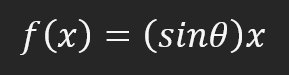
So, we can assume that the required constant is the sine of the angle, and thus compose our equation. However, this is not the case. Not because the constant is unrelated to the angle (in fact, it is), but because you would think you would use the sine or cosine. This method is not the best general way to express the idea. Usually, an affine equation is not expressed in trigonometric functions. This is not wrong, this is just unusual. In this article, we will see how the angle can be used to obtain this constant. However, first I need to explain something else. If you change the code a little, as shown in the code below, you can see that it will look more like the correct equation of the line shown in the animation. Because the constant will know use the correct term.

35. //+------------------------------------------------------------------+
36. void NewAngle(const char direct, const double step = 1)
37. {
38.     canvas.Erase(ColorToARGB(clrWhite, 255));
39.     Func_01();
40. 
41.     global.Angle = (MathAbs(global.Angle + (step * direct)) < 90 ? global.Angle + (step * direct) : global.Angle);
42.     canvas.TextOut(global.x + _SizeLine + 50, global.y, StringFormat("%.2f", MathAbs(global.Angle)), ColorToARGB(clrBlack));
43.     canvas.TextOut(global.x, global.y + _SizeLine + 50, StringFormat("f(x) = %.2fx", -MathTan(_ToRadians(global.Angle))), ColorToARGB(clrBlack));
44.     canvas.Line(
45.                 global.x - (int)(_SizeLine * cos(_ToRadians(global.Angle))), 
46.                 global.y - (int)(_SizeLine * sin(_ToRadians(global.Angle))), 
47.                 global.x + (int)(_SizeLine * cos(_ToRadians(global.Angle))), 
48.                 global.y + (int)(_SizeLine * sin(_ToRadians(global.Angle))), 
49.                 ColorToARGB(clrForestGreen)
50.             );
51.     canvas.Update(true);
52. }
53. //+------------------------------------------------------------------+

The result of the code execution is shown in the gif image below.

Notice that now, thanks to line 43, we have something very close to the equation of a straight line. You can see that to create the formula, we will use the tangent of the angle, and not the sine or cosine. This is just an attempt to generate the most appropriate value. However, although we manage to formulate the equation, we can see that it is not so easy to guess the optimal value of the slope of the line, that is, the angle of the system. We can try to do it manually, but it is a very difficult task. Despite all the complexities of constructing the equation that produces linear regression, it is important to remember that at this point we are working with only one variable in this system. This is the value we need to find, as shown in the animation above.

However, if we use mathematics correctly, it will allow us to find the most appropriate value for the slope angle. For this, we will need to use derivatives in our system. We also need to understand why tangent is the trigonometric function that best indicates the constant to be used in the equation. But to make this easier to understand, my dear reader, let's start a new topic.

Using derivatives

This is where the math gets a little confusing for many. But it is not a cause for despair, fear or affliction in hearts. We need to tell our code how to find the optimal value for the angle so that the equation allows us to access values we already know or get as close to them as possible. Thus, the equation will have constants with the values very close to ideal. This will allow the knowledge present on the graph to be preserved in the equation format, which in this case will be a linear equation.

The fact that we work with a linear equation, which often resembles linear regression, is because this type of equation is the easiest for calculating the necessary constants. This is not because it is a better way to represent values on a graph, but because it is easier to calculate. However, in some cases the processing time may be significant. But that's a separate question.

To compute such an equation, we need some mathematical resources. This is because an affine function is a straight line function and does not allow us to obtain a derivative. A derivative is a straight line passing through a given point and it can be obtained from any equation. Many people get confused by these explanations, but, actually, a derivative is just a tangent line at a given point of the function. The tangent line is drawn at a point belonging to the equation that usually creates the curve on the graph. Since the affine function is a tangent line, the tangent reflects the value of the constant by which the unknown part is multiplied, providing the equation of that specific line. For this reason, the second tangent cannot be drawn using this original equation. We need something else for this. Thus, it does not matter which point we try to use to obtain the derivative. It is not possible to create a derivative in an affine function.

However, there is a way to ensure the creation of a derivative. This is exactly what we will begin to study today. To understand how we will do this, you need to understand what a derivative is. Then you will need to understand the method used to obtain this derivative and, accordingly, to create an affine function describing a minimally ideal line. To do this, we will use a function that allows us to output the derivative. The simplest of them is the quadratic function. Its formula is shown below:

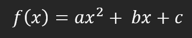
Note that there is a power of two in this equation. This fact alone allows us to explain the presence of a derivative in the system, but we can use any function to construct the curve. It could even be a log function. However, a log function won't make sense if we look at what we need to do next. For this reason, and to make the process as simple as possible, we will use a quadratic equation. Thus, using the above formula, we get the following graph.

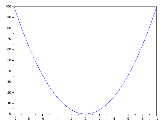
This graph is achieved by setting the value of A to one, and the values of B and C equal to zero. However, what is really important for us is the curve that can be seen on the graph.

Now pay attention - this explanation is important for understanding what we will implement in our program to find the equation we need.

From the graph above, we will make some assumptions, and it is important to understand them. We want to know the value of the derivative at the point where X is equal to four. To do this, you need to draw a tangent line that must exactly pass through the point where X is equal to four. At first glance, this is simple: take a ruler and mark a point X on the coordinate equal to four. And then we will try to construct a line tangent to a point on the curve. But can we actually draw a tangent line by doing this? This is unlikely!

It is much more likely that we will create a line that will not be tangent. For this reason, we need to do some calculations. This is where things get complicated. But in order not to complicate the situation for no reason, I will not go into details of the calculations themselves at this stage. I assume that the reader knows the formula for the derivative of a quadratic equation. For those who don't know, I will explain later how to get this formula. What's important for us now is the way of obtaining derivative equations. The final result is not that important, but the formula obtained from the derivative is important. So let's continue.

The derivative of a quadratic equation can be found using the following formula.

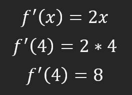
Next I will show two of the most common notations. You can use the one on the right or the one on the left, it doesn't matter. Now we are interested in the formula itself, it is equal to 2 times X. This formula gives us a value of eight, which in our example is the value of the tangent line at the point where X is four. If you know what the value eight means, you can draw a tangent line at the point where X equals four. However, if you don't know what this value means, you will need a second formula to plot the tangent. 

If you don't understand why the value is eight, look at the picture below where we want the derivative with respect to X to be four. To do this, we calculate the value at that position as shown below.

But before we move on to other calculations, let's figure out what this value eight means. It means that if we move one position on the X axis, we need to move eight positions on the Y axis. And this will allow us to draw a tangent line. You may not believe it until you see it happen in real life. If this is your case, there is a formula that allows you to write the equation of a tangent line. This equation is:

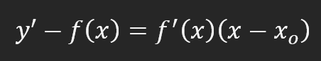
Yes, it's a little scary, but it's much simpler than it seems. Although, this formula is definitely quite special. It allows you to create an equation of a tangent to a derivative, although the derivative will ultimately be a tangent line. But this is just a fact that I mention as something interesting, nothing to worry about. So, since we already know most of the values, we can make the appropriate substitutions to find the formula for the equation of the tangent line. This moment can be seen below.

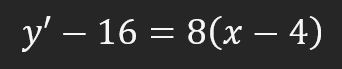
This is where a lot of the complexity comes in, but let's figure out where these values come from. The value 16 is the result of the original equation. In other words, we substituted into the quadratic equation the value of X that we use in the derivative, that is, "4". The value 8 is obtained as a result of calculating the derivative of the function. Again, X is equal to 4, and this also applies to the derivative of the function. The value 4 we see here is the initial value of X that we use in all the other equations. After the calculations, we obtain the following formula for the tangent line.

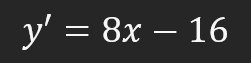
Great, now we can draw a tangent line based on the equation above. The drawn line can be seen in the image below, it is highlighted in red.

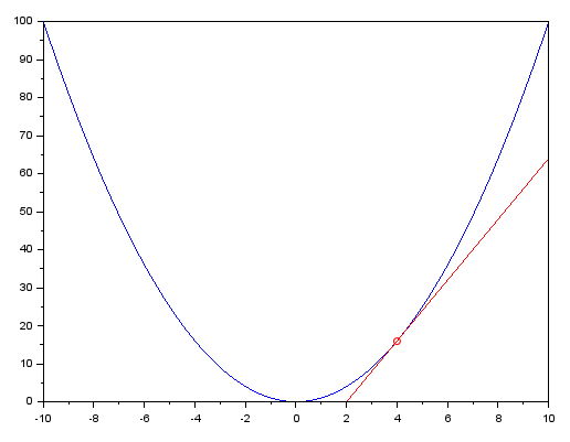
This graph was created using the SCILAB program. For those who want to take a closer look, below is the code used in SCILAB to generate it.

x = [-10:.2:10];
y = x ^ 2;

plot(x, y, 'b-');
plot(4, 16, 'ro');

x = [2:.2:10];
y = 8 * x - 16;

plot(x, y, 'r-');

I am adding this so that you can understand that it is not just about learning how to use this or that program. Being proficient in a particular language is not what gives you real qualifications. Often we have to resort to various programs in order to analyze the situation with accuracy. For this reason, further education is of great importance. And no matter how good you think you are, there will always be someone more experienced than you in one area or another. So, always learn.

Now we have all the necessary knowledge, but what does this tangent line mean? And why is it so important for those who work with neural networks? The reason is that this line shows us where we should move. More precisely, where our program should move to create a linear regression equation.

But that's not all: this line explains how to calculate deviations. It is in these calculations that the "magic" of neural networks lies. Can't you see it? Perhaps, you can't understand how this is possible. So, to understand this, we need to understand what drives the derivative calculation. Even though we use the tangent line at the end, the calculations do not arise from the tangent line. They arise from another trigonometric function. This is where the magic of the system lies. This "magic" allows us to create a general solution for all possible and acceptable cases, which is what makes the neural system work. So we'll leave that for another topic to keep things separate.

Secant line

Although when everyone talks about neural networks, they only mention derivatives, the secret is not in the derivative or the tangent line. The secret lies in another straight line. And this is a secant line. That is why there was a certain reluctance on my part to write on the topic of neural networks. In fact, people were asking me to cover this topic. The truth is that a lot of people talk about neural networks, but very few actually understand how they work from a mathematical perspective. Programming is the easy part, the hard part is math. Many people believe that they should use this or that library, this or that programming language. But in reality, we can use any language if we understand how its mathematical component works. I don't mean to speak negatively about anyone or to suggest that anyone is wrong in their explanations. Everyone has the right to understand everything the way they want. However, my desire is to truly explain how everything works. I don't want you to become another slave to languages or libraries. I want you to understand how everything works from the inside. That's why I decided to write a series of articles to talk about this topic.

The idea behind the derivative is to find the value of the tangent line. This happens because the tangent line indicates the slope of the function. In other words, it is the error of linear regression when used in a neural network. Therefore, when the tangent line begins to reach an angle of zero degrees, the error will approach zero. In other words, the equation that generates linear regression on the values already existing in the database approaches the ideal values. This is what happens in this particular case and with these particular values.

However, when we perform the computations, we do not use the tangent line. We actually use a secant line. It does not matter what kind of neural network is implemented. If there is a computation, then not a tangent line but a secant line is used. You might think that this is much more complicated, but if you think that, then you don't know how the tangent line to the derivative is actually obtained. Or, even worse, how the formula for the derivative is obtained. There is no particular point in memorizing formulas. The best thing to do is to understand why the formula has this format and not another. Remember the calculations given in the previous topic? Do you know where they came from? If not, let's look at the graph below:

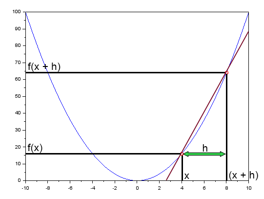
The red line on this graph is a secant line. If you have been attentive so far, now I want you to double your attention. This will be even more important than anything else you can read or hear about neural networks.

Here I use the same X point as in the previous topic, it's equal to 4. I do this to help you better understand what I am explaining.

Note that it is impossible to generate a tangent line, no matter what you think or imagine. It is impossible to generate a tangent lien from a curve on a graph.. However, if you use a secant line, you can get a tangent. How? It's all very simple. Note that f(x + h) is f(x) shifted by a distance h. Then, if h tends to zero, the secant will turn into a tangent. And when h is exactly zero, the secant line shown in the figure will exactly coincide with the tangent. So, at this point, the tangent line will give us the slope of the derivative of the function at the given point. Okay, but I still don't understand. Well, my dear reader, let's put what you see above in a less confusing form, perhaps that will clarify the situation.

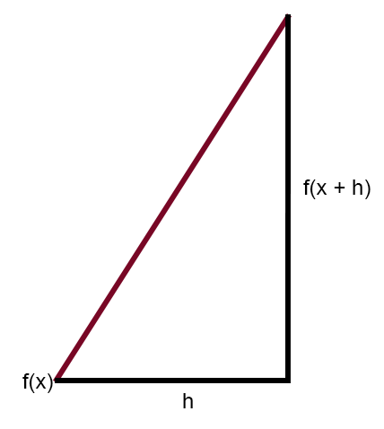
The image above shows the same thing as the previous one. I think this will make the idea of using the secant clearer. And why, unlike what everyone claims, that we use a tangent line or derivatives when we use a neural network, we actually use a secant line so that the computer can generate the correct equation.

If you decrease the value of h, you will start approaching f(x), but this h will never be equal to zero. This is when we are using neural networks. This may be a very small value; how small this value is depends on one thing, which we will see later. This moment is known as neural network madness. The smaller this value h is, the less crazy the neural network will be, but the larger it is, the crazier it will be. Why? The reason is convergence. During the computations that we will consider later, it will be possible to notice that this convergence tends to the value h. This will result in the equation obtained at the end tending to vary within this convergence. For this reason, h is very important. The explanation seems complicated, but you will see that everything is much simpler in practice. However, we have not yet reached the point we want to show. Based on the image above, we get the following formula.

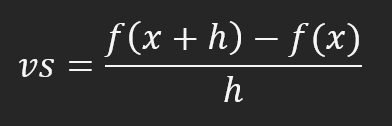
This formula shows how far the secant line is from the tangent line. However, in the calculation actually used is the one shown in the figure below.

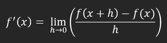
This equation explains everything you need to know about neural networks. This is why they say that neural networks use derivatives. It is this equation that generates the calculations that many simply memorize: derivative formulas. That's it. There is nothing more to be explained or discussed. All we need is this equation shown above. With this, I can close the article and go live my life quietly.

Final thoughts

But wait a minute. You have not explained how to use this secant equation, or why it explains everything. What do you mean, "have not explained"? Are you kidding me? Dear reader, in fact, I have just started introducing this topic. I want you to study this material calmly first. In the next article on neural networks, we will look at how to use the knowledge presented here to formulate the correct equation.