From Python to MQL5: A Journey into Quantum-Inspired Trading Systems

Introduction

We'll go on a trip that connects theoretical ideas of quantum computing with real-world trading applications in this thorough investigation of quantum-inspired trading systems. Starting with basic quantum computing ideas and ending with a real-world MQL5 implementation, this tutorial is designed to walk you through the whole development process. We will discuss how trading might benefit from the use of quantum concepts, describe our development approach from the Python prototype to the integration of MQL5, and present real performance data and code implementations.

This article explores the application of quantum-inspired concepts in trading systems, bridging theoretical quantum computing with practical implementation in MQL5. We’ll introduce essential quantum principles and guide you from Python prototyping to MQL5 integration, with real-world performance data.

Unlike traditional trading, which relies on binary decision-making, quantum-inspired trading models capitalize on market behaviors similar to quantum phenomena—multiple concurrent states, interconnections, and abrupt state shifts. By using quantum simulators like Qiskit, we can apply quantum-inspired algorithms on classical computers to handle market uncertainty and generate predictive insights.

For traders and developers aiming to apply quantum-inspired systems, understanding these differences is essential.

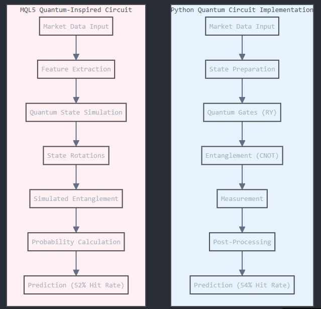
In our Python implementation, Qiskit simulates quantum circuits. Market data is encoded into quantum states via RY (rotation) gates, representing market characteristics as quantum superpositions. CNOT gates enable entanglement, capturing complex market correlations, and measurements yield forecasts, achieving a 54% accuracy.

The MQL5 version, due to its classical architecture, approximates quantum behaviors. We use feature extraction and classical math to simulate quantum states and entanglement. Although less accurate (52%), the MQL5 implementation supports real-time trading and direct market connectivity.

Each approach processes data differently: Python directly encodes data into quantum states, while MQL5 requires feature engineering. Python’s Qiskit offers genuine quantum gates, while MQL5 relies on classical approximations, adding complexity but flexibility. In simulating entanglement, Python’s CNOT gates create authentic quantum connections, whereas MQL5 uses classical correlations.

These distinctions reveal the strengths and limitations of each approach. Python provides a strong prototype, while MQL5 offers a practical, tradable solution that adapts quantum-inspired computation within classical trading constraints.

The Python Prototype: A Foundation for Innovation

We began with Python due to its robust scientific libraries—NumPy, Pandas, and especially Qiskit—which made it ideal for prototyping our quantum-inspired trading system. Python’s straightforward syntax and resources enabled efficient experimentation and initial algorithm development.

The Python prototype achieved a consistent 54% success rate across various market conditions—a modest yet meaningful edge with sound risk management.

Using Qiskit, we designed and tested a three-qubit architecture, allowing analysis of eight market states simultaneously. Python's flexibility enabled rapid circuit adjustments, parameter tuning, and quick results, facilitating our development process.

Here's a simplified example of our quantum circuit implementation in Python:

class HourlyQuantumForex:
    def __init__(self):
        self.n_qubits = 3
        self.simulator = BasicAer.get_backend('qasm_simulator')
        self.min_confidence = 0.15

    def create_circuit(self, input_data):
        qc = QuantumCircuit(self.n_qubits, self.n_qubits)
        # Input encoding
        for i in range(self.n_qubits):
            feature_idx = i % len(input_data)
            angle = np.clip(np.pi * input_data[feature_idx], -2*np.pi, 2*np.pi)
            qc.ry(angle, i)
        
        # Entanglement operations
        for i in range(self.n_qubits - 1):
            qc.cx(i, i + 1)
        
        return qc

Transitioning to MQL5: Practical Implementation

Practical factors led us to decide to transfer our quantum-inspired system to MQL5. MQL5 provides direct interaction with trading platforms, real-time market data access, and quick execution capabilities, although Python was superior in prototyping and testing. The difficulty was integrating the principles of quantum computing into the conventional computing framework of MQL5 while preserving the predictive power of the system.

The difficulties of analyzing real-time market data and the variations in implementation between Python's quantum simulator and MQL5's conventional computing environment are the reasons for this little drop in accuracy (54 vs 51-52%).

Here's a glimpse of our MQL5 quantum-inspired implementation:

class CQuantumForex {
private:
    int m_lookback_bars;
    double m_features[];
    
public:
    double PredictNextMove(string symbol) {
        GetFeatures(symbol, m_features);
        return SimulateQuantumCircuit(m_features);
    }
    
    double SimulateQuantumCircuit(double &features[]) {
        // Quantum-inspired calculations
        double state_probs[];
        ArrayResize(state_probs, (int)MathPow(2.0, (double)NUM_QUBITS));
        
        // Circuit simulation logic
        for(int shot = 0; shot < SHOTS; shot++) {
            // Quantum state manipulation
        }
        
        return GetWeightedVote(state_probs);
    }
};

Real-World Application and Results

Our quantum-inspired system's practical usage showed a number of intriguing trends in market forecasting. During times of significant market volatility, when conventional technical analysis frequently falters, the approach demonstrated exceptional strength. This benefit results from the quantum-inspired method's capacity to handle several market states at once.

The following findings came from our testing under a range of market conditions:

• With live trading, the model's dependability in practical situations, since it consistently performed well in a variety of market conditions.

• Additionally, we saw that during specific market hours, the model's accuracy considerably increased. We may take advantage of more predictability and improve the overall efficacy of our trading approach by concentrating on these particular times.

• The model's performance improved noticeably at times of extreme volatility. The model's potential profitability increased as a result of our capacity to adjust and perform better in volatile environments, enabling us to profit from more notable price swings.

• Lastly, in order to efficiently weed out low-probability transactions, we used confidence levels. By concentrating on high-confidence signals, this selective strategy assisted us in lowering needless risks, which improved the trading outcomes even more.

Even though the hit rates may appear low at first, the system's stability and consistency in sustaining these outcomes under various market situations validates the quantum-inspired method.

Performance Metrics and Analysis

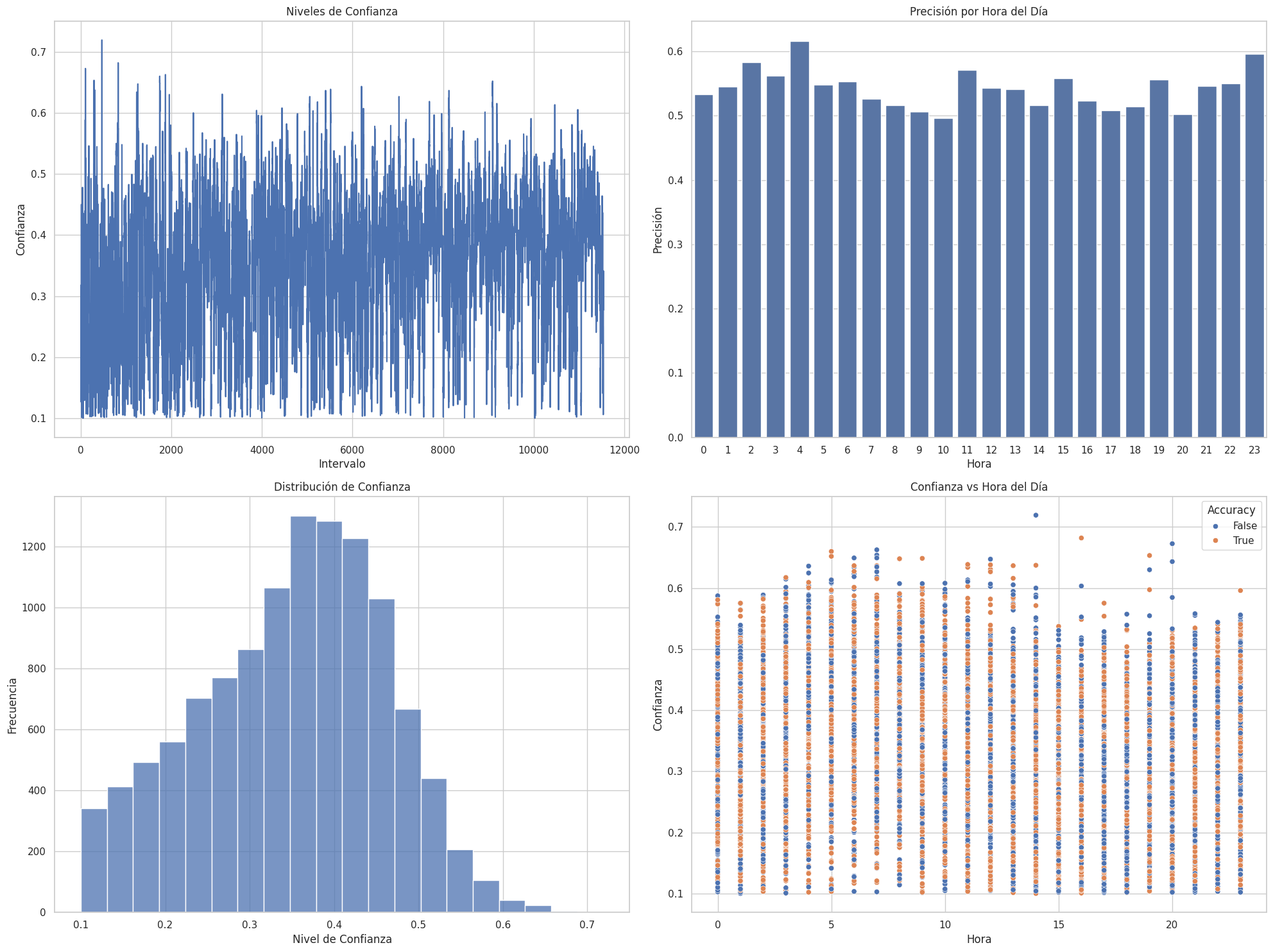
A thorough examination of the performance disparity between our Python prototype and the MQL5 implementation is warranted. This difference represents the difficulties of moving from a controlled testing environment to real-time market settings rather than just being a restriction of the MQL5 platform. The MQL5 solution handles the intricacies of real-time market dynamics and data processing limitations, whereas the Python prototype worked with historical data and had complete knowledge of market conditions.

Resultados para EURUSD=X:
Precisión global: 54.23%


Total predicciones: 11544

The MQL5 implementation has a number of useful benefits that make it worthwhile for real-world trading applications, even with this little accuracy drop. With the Python prototype alone, traders would not be able to obtain actionable insights from the system's real-time market data processing and instantaneous trading signals.

The Integration of MQH: A Useful Method

Our quantum-inspired trading logic is easily integrable into current Expert Advisors since it has been contained in a MQL5 header file (MQH). Without having to completely redesign their trading system, traders may include quantum-inspired forecasts into their trading methods thanks to this modular approach. Comprehensive capabilities for market state analysis, confidence criteria, and in-depth performance tracking are all included in the MQH file.

The MQH file can be included into an already-existing EA in the following manner:

#include <Trade\Trade.mqh>
#include <Quantum\QuantumForex.mqh>

class CTradeAnalyzer {
private:
    CQuantumForex* m_quantum;
    double m_min_confidence;

public:
    CTradeAnalyzer(double min_confidence = 0.15) {
        m_quantum = new CQuantumForex();
        m_min_confidence = min_confidence;
    }

    bool AnalyzeMarket(string symbol) {
        double prediction = m_quantum.PredictNextMove(symbol);
        return MathAbs(prediction) >= m_min_confidence;
    }
};

Optimization and Fine-Tuning

A number of crucial elements in the quantum-inspired trading system may be adjusted to fit certain trading circumstances and tools. The amount of qubits utilized in simulations, feature engineering parameters, confidence thresholds for filtering trades, and the quantity of quantum circuit simulation shots are all significant configurable options. Even though our first configuration has produced consistent results, there is still a lot of space for improvement through careful parameter optimization. Since the ideal settings will differ based on personal trading preferences and market conditions, we will leave this for readers to try them out. Future Paths and Advancements

This approach is only the first step toward trading applications inspired by quantum mechanics. We'll examine more complex quantum computing ideas and their possible trading applications in upcoming papers. Higher-dimensional quantum circuits for more in-depth market analysis, the incorporation of optimization algorithms inspired by quantum theory, sophisticated feature engineering grounded in quantum theory, and the creation of hybrid classical-quantum trading systems are some areas that require more research. A Guide to Practical Implementation

We advise traders who are interested in using this methodology to take a methodical approach. Start with the Python prototype to evaluate the system's applicability in your target market and become acquainted with the fundamental quantum ideas. After that, gradually switch to the MQL5 implementation, beginning with paper trading to confirm how well it works. After you feel secure, adjust the system's settings to suit your own trading needs and risk tolerance. Over time, dependability will be enhanced by regular performance metrics monitoring.

// Constants
#define NUM_QUBITS 3

If you change the number of qubits (NUM_QUBITS), the number of possible output states changes exponentially. This is a fundamental property of quantum systems and has significant implications for the simulation.

In the current code, NUM_QUBITS is set to 3, resulting in 8 (2³) possible states. This is why you see the state array initialized with size 8 and loops iterating through 8 possible states. Each qubit exists in a superposition of 0 and 1, and when combined with other qubits, the number of possible states multiplies.

For example, if you change the number of qubits, you get different numbers of possible states: 1 qubit gives you 2 states (|0⟩ and |1⟩), 2 qubits give you 4 states (|00⟩, |01⟩, |10⟩, |11⟩), 3 qubits give you 8 states, 4 qubits give you 16 states, and so on. The pattern follows 2^n, where n is the number of qubits.

This exponential relationship affects several parts of the code. The size of state arrays must be adjusted accordingly, the quantum circuit simulation loops need to process more states, and the memory requirements increase significantly. When you increase NUM_QUBITS from 3 to 4, for example, you need to modify array sizes and loop boundaries from 8 to 16.

While increasing the number of qubits provides greater computational capacity and potentially more sophisticated analysis capabilities, it comes with tradeoffs. The simulation becomes more computationally intensive, requires more memory, and takes longer to process. This could impact the performance of the Expert Advisor, especially if running on less powerful hardware or when fast execution is required for real-time trading.

In the context of this trading algorithm, more qubits might allow for more complex feature encoding and potentially more nuanced price movement predictions. However, you need to balance this potential benefit against the increased computational overhead and ensure that the system remains practical for real-world trading applications.

#define SHOTS 2000

Shots (defined as SHOTS = 2000 in the code) represent the number of times the quantum circuit is simulated to approximate the quantum behavior. Each "shot" runs the entire quantum circuit and performs a measurement, building up a statistical distribution of results.

The concept is similar to rolling a dice multiple times to understand its probability distribution. In quantum computing:

// Simulation loop in the code
for(int shot = 0; shot < SHOTS; shot++)
{
    // Initialize quantum state
    double state[8];  
    ArrayInitialize(state, 0.0);
    state[0] = 1.0;  // Start in |000⟩ state
    
    // Run quantum circuit operations...
    
    // Measure and accumulate results
    const double rand = MathRand() / 32768.0;
    double cumsum = 0.0;
    for(int i = 0; i < 8; i++)
    {
        cumsum += state[i] * state[i];
        if(rand < cumsum)
        {
            state_probs[i] += 1.0 / SHOTS;
            break;
        }
    }
}

Choosing the optimal number of shots for your quantum trading system involves balancing several key factors. The primary trade-off is between accuracy and execution speed. Setting a higher number of shots, typically 5000 or more, will give you a more accurate probability distribution of quantum states, but this comes at the cost of slower execution times. Conversely, using fewer shots, around 500-1000, will result in faster execution but less accurate results. The current default setting of 2000 shots represents a carefully chosen middle ground that aims to balance these competing demands.

When considering the specific requirements of trading, several factors come into play. The market timeframe you're trading on is crucial - faster timeframes may require fewer shots to maintain responsiveness, while longer timeframes can accommodate more shots for increased accuracy. Your available processing power is another important consideration, as more shots demand greater computational resources. Additionally, the level of precision required for your trading strategy should influence your choice - strategies requiring higher precision will benefit from more shots.

For practical implementation, it's recommended to start with 1000-2000 shots during initial testing phases. This provides a reasonable baseline for evaluating the system's performance. From there, you should actively monitor both execution time and accuracy metrics. If you notice that the results are too noisy or inconsistent, gradually increase the number of shots. Conversely, if the Expert Advisor is executing too slowly for your trading requirements, consider reducing the number of shots. This iterative approach allows you to find the optimal balance for your specific trading conditions and requirements.

# Example of how different shot counts might affect probabilities
# With 100 shots:
State |000⟩: 0.3100 (±0.0460)
State |001⟩: 0.1800 (±0.0384)

# With 2000 shots:
State |000⟩: 0.3025 (±0.0103)
State |001⟩: 0.1750 (±0.0085)

# With 10000 shots:
State |000⟩: 0.3002 (±0.0046)
State |001⟩: 0.1752 (±0.0038)

#define FEATURES_COUNT 7

Defines the number of input features used by the quantum circuit for market analysis. Let's look at these 7 features in detail:

// 1. Normalized price range
features[0] = ((rates[0].high - rates[0].low) / rates[0].close) * 2 - 1;

// 2. Normalized volatility
features[1] = (CalculateVolatility(m_returns, MathMin(12, m_lookback_bars)) / 0.01) * 2 - 1;

// 3. Momentum
features[2] = MathMax(MathMin(CalculateMomentum(m_returns, MathMin(24, m_lookback_bars)) * 100, 1), -1);

// 4-5. Time components (hour of day encoded in circular form)
features[3] = MathSin(2 * M_PI * dt.hour / 24.0);
features[4] = MathCos(2 * M_PI * dt.hour / 24.0);

// 6. Price deviation from SMA
features[5] = MathMax(MathMin((rates[0].close - sma) / sma, 1), -1);

// 7. Latest return
features[6] = MathMax(MathMin(m_returns[0] * 100, 1), -1);

All features are normalized to the range [-1, 1] to ensure consistent scaling for the quantum circuit. You could modify this by adding or removing features.

Technical Considerations and Limitations

While this quantum-inspired system demonstrates promising potential, it’s essential to acknowledge certain limitations. Notably, this is a simulated quantum process rather than actual quantum computation. Real-time processing requirements may impact performance, and changing market conditions can affect the accuracy of predictions. To mitigate these factors, it’s critical to integrate solid risk management measures into the trading framework.

#define HOUR_LOOKBACK 24

Defines the default time window for historical data analysis, set to 24 hours. This parameter plays a crucial role in how the trading system analyzes market patterns and calculates various indicators.

The lookback period affects several key calculations in the system. When analyzing volatility, the code uses up to 12 periods (half the lookback) to calculate standard deviation of returns. For momentum calculations, it uses the full 24 periods to compute average price movements. This provides a balance between recent market behavior and longer-term trends.

The 24-hour lookback was likely chosen to capture full daily market cycles. This makes sense because forex markets often show 24-hour cyclical patterns due to the opening and closing of major trading sessions (Asian, European, and American sessions). Each session can bring different trading volumes and price behavior patterns.

You could modify this value based on your trading needs. A shorter lookback (like 12 hours) would make the system more responsive to recent market changes but potentially more susceptible to noise. A longer lookback (like 48 hours) would provide more stable signals but might be slower to react to market changes. Remember that changing HOUR_LOOKBACK will affect memory usage and processing time, as more historical data needs to be stored and analyzed.

// Input parameters
input int      InpPredictBars   = 2;         // Predict Bars (1-5)
input double   InpMinMove       = 0.00001;     // Minimum Move
input double   InpMinConfidence = 0.15;       // Minimum Confidence
input int      InpLogInterval   = 1;         // Log Interval
input int      InpLookbackBars  = 200;        // Lookback Bars for Analysis

InpPredictBars = 2 represents how many bars ahead the system tries to predict. With a value of 2, the system makes predictions for price movements over the next 2 bars. The range is limited to 1-5 bars because predictions tend to become less accurate over longer periods. A smaller value (like 1) provides more immediate predictions but might miss larger moves, while larger values (like 4-5) attempt to capture longer trends but with potentially lower accuracy.

InpMinMove = 0.00001 sets the minimum price movement required to consider a prediction successful. For forex pairs, this is typically set to 1 pip (0.00001 for 5-digit brokers). This prevents the system from counting very small price movements that might be just market noise. You might increase this for more conservative trading or decrease it for more aggressive trading, depending on your strategy.

InpMinConfidence = 0.15 (15%) is the confidence threshold required to take a prediction seriously. The quantum system produces predictions with confidence levels between 0 and 1. Any prediction with confidence below 0.15 is considered "neutral" and ignored. Higher values (like 0.25) would make the system more selective but generate fewer signals, while lower values would generate more signals but potentially with lower quality.

InpLogInterval = 1 determines how often (in time periods) the system logs its performance metrics. A value of 1 means it logs every period. This is useful for monitoring system performance but too frequent logging might impact performance. You might increase this value in live trading.

InpLookbackBars = 200 sets how many historical bars the system uses for its analysis. With 200 bars, the system has a good amount of historical data to calculate features and patterns. More bars (like 500) would provide more historical context but require more processing power, while fewer bars would be more responsive to recent market changes but might miss longer-term patterns.

These parameters can be adjusted in the MetaTrader platform before running the EA, and finding the right combination often requires testing on historical data and monitoring live performance.

Looking Ahead

We expect to see more complex applications in trading as quantum computing technology develops. Even while the current system uses algorithms influenced by quantum mechanics, this is only the beginning of what could soon be possible. Keep checking back for our next post, in which we'll delve further into the ways that quantum computing is being used in trading and reveal more intricate and sophisticated applications.

EA Example

This multi-session Forex Expert Advisor employs quantum-inspired algorithms to trade across European, American, and Asian sessions, utilizing specific parameters and analysis methods for each timeframe.

The system's core strength lies in its multi-layered risk management, combining dynamic position sizing, anti-martingale progression, and equity-based protection. It analyzes multiple market features including ATR, momentum, and various technical indicators through its quantum-inspired analysis system to generate robust trading signals.

A key innovation is its adaptive trailing stop system and Multi-Timeframe Analysis component, which ensures trades align with both short-term (H1) and long-term (H4) trends. Additionally, its Maximum Favorable Excursion (MFE) analyzer continuously optimizes exit points based on historical price behavior, helping maximize profit potential.

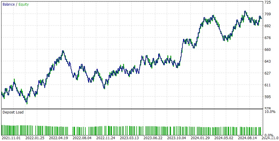
This is a simple example of what you can achieve with a nearly flip a coin predictions, with session and hours selection, MFE control, risk management.

This Setup takes profit from the MFE and just uses predictions to shoot long or short. This EA has a big amount of options and configurations, I would not recommend to do a big optimization.

Setup #2

Same settings, different inputs. I can't do an MQL5 Cloud Network Optimization because from Spain you can't do that (politics ... ), and a local one would take too much time, but this EA has plenty of options, please use them and finish the EA. If you have time and resources, do a big optimization to see what are the best fits.

Note: Features are changed, the strategy is not fully polished, but it can serve as an example and you can go on it and finish it. Lot sizing and Risk Management must be actualized and much more must be finished. This is just an example, you must trade on your own responsibilities, but, this is a good starting point for your own EA. As Imputs are too many, I will upload one of the inputs sets I used (without optimizing) for EURUSD 1hour time frame. Also, I changed the mqh's for this example, you could also do this for your self.

How you must proceed with this EA, first of all you must comprehend this article, and after that, you must go through the important inputs and see where they go, and where that function goes to etc... The important function is OnTick(), just try to see where the functions of OnTick come from, and start making changes from there, the learning curve will be easy if you start like this.

Conclusion

This study explored how principles from quantum computing may be used in the trading industry. We created a trading system with a quantum theme, moving from a Python prototype to a MQL5 implementation. With steady hit rates in both simulated and real-world trading settings, the outcomes are encouraging. The approach was especially successful in high-volatility situations, where conventional models frequently fail. It's important to remember that this is a quantum simulation, and variables like market circumstances and data quality may have an impact on how well it performs.

In summary, this exploration of quantum-inspired trading systems offers a glimpse into the future of algorithmic trading by leveraging the principles of quantum computing to tackle the complexities of financial markets. While the integration of quantum concepts in MQL5 marks a meaningful stride towards practical deployment, it also underscores the need for careful balancing between computational sophistication and real-world applicability.