Population optimization algorithms: Resistance to getting stuck in local extrema (Part II)

Contents

1. Algorithms
2. Improving agent for BGA
3. Conclusions

As part of our research, we delve into the study of the robustness of population optimization algorithms, and their ability to overcome local traps and achieve global maxima on a variety of test functions. In the previous article, we looked at algorithms that showed modest results in the ranking. Now it is time to pay attention to the top performers.

We strive to conduct an in-depth analysis of each of these algorithms, while identifying their advantages and unique features. Our goal is to understand what strategies and approaches make these algorithms successful in overcoming complexity and achieving global optimization goals.

This research stage will allow us to not only better understand the resilience of population algorithms to getting stuck in local traps, but also to identify the key factors that contribute to their success in the face of diverse and complex test functions. My efforts aim to increase understanding of how these algorithms can be optimized and improved, and to identify opportunities for their joint use and hybridization to effectively solve various optimization problems in the future.

1. Algorithms

Let's continue studying the algorithms that occupy the top positions in our comparison table. They definitely deserve more detailed consideration and attention. Let's dive into a detailed analysis of their features to uncover all the aspects that make them so valuable and effective in solving complex optimization problems.

Below are reports of the algorithms operation, which should be read as follows:

• C_AO_FSS:50;0.01;0.8             - algorithm name and external parameters
  
• 5 Hilly's                                   - name of the test function and its number in the test
  
•  Func runs: 10000                   - number of runs
  
• result: 0.32457068874346456  - obtained result, where 0.0 is the minimum of the test function, and 1.0 is the maximum. The higher the value, the better
  
• All score: 1.33084                   - total value of the points scored. The higher the value, the better

Evolutionary strategies, (P+O)ES

C_AO_(P_O)ES:100:150:0.02:8.0:10
=============================
5 Hilly's; Func runs: 10000; result: 0.45574011563217454
25 Hilly's; Func runs: 10000; result: 0.5979154724556998
500 Hilly's; Func runs: 10000; result: 0.3415203622112476
=============================
5 Forest's; Func runs: 10000; result: 0.18929181937830403
25 Forest's; Func runs: 10000; result: 0.1837517532554242
500 Forest's; Func runs: 10000; result: 0.15411134176683486
=============================
5 Megacity's; Func runs: 10000; result: 0.10153846153846155
25 Megacity's; Func runs: 10000; result: 0.12030769230769231
500 Megacity's; Func runs: 10000; result: 0.08793846153846216
=============================
All score: 2.23212

Unlike its younger brother (PO)ES, (P+O)ES is highly active in the search space, especially on the smooth Hilly function, where the population is divided into several groups, each of which explores different areas. However, for some reason its efficiency decreases on the smooth Forest function, while on the discrete function it performs poorly (only the nearest hill is reached). In general, the algorithm is very interesting on smooth differentiable functions, but there is a clear tendency to get stuck. Besides, it lacks capabilities that refine the result.

Grey Wolf Optimizer (GWO)

C_AO_GWO:50;10
=============================
5 Hilly's; Func runs: 10000; result: 0.5385541648909985
25 Hilly's; Func runs: 10000; result: 0.33060651191769963
500 Hilly's; Func runs: 10000; result: 0.25796885816873344
=============================
5 Forest's; Func runs: 10000; result: 0.33256641908450685
25 Forest's; Func runs: 10000; result: 0.2040563379483599
500 Forest's; Func runs: 10000; result: 0.15278428644972566
=============================
5 Megacity's; Func runs: 10000; result: 0.2784615384615384
25 Megacity's; Func runs: 10000; result: 0.1587692307692308
500 Megacity's; Func runs: 10000; result: 0.133153846153847
=============================
All score: 2.38692

A pack of wolves of the GWO algorithm rushes across the vast expanses of the virtual world, rapidly spreading in all directions on various test functions. This property can be effectively used in the initial iterations, especially if the algorithm is paired with another method that can improve and complement the solutions found. The pack's excellent research abilities speak of their potential, but unfortunately, accuracy in identifying areas remains their weak point. Interestingly, the algorithm showed even better results than in the conventional test with the uniform distribution of agents.

Shuffled Frog-Leaping algorithm (SFL)

C_AO_SFL:50;25;15;5;0.7
=============================
5 Hilly's; Func runs: 10000; result: 0.5009251084703008
25 Hilly's; Func runs: 10000; result: 0.3175649450809088
500 Hilly's; Func runs: 10000; result: 0.25514153268631673
=============================
5 Forest's; Func runs: 10000; result: 0.4165336325557746
25 Forest's; Func runs: 10000; result: 0.21617658684174407
500 Forest's; Func runs: 10000; result: 0.15782134182434096
=============================
5 Megacity's; Func runs: 10000; result: 0.2892307692307692
25 Megacity's; Func runs: 10000; result: 0.14892307692307696
500 Megacity's; Func runs: 10000; result: 0.10636923076923148
=============================
All score: 2.40869

The SFL algorithm demonstrated an even wider range of propagation capabilities in different directions of the search space, even on a discrete Megacity function, compared to the previous algorithm in the list. SFL is capable of reaching even global maximum regions within a given number of iterations. However, the accuracy of refining the solutions found is not SFL's strong point. Similar to GWO, the algorithm demonstrated results that were superior to those in conventional testing.

Random Search Algorithm (RND)

C_AO_RND:50
=============================
5 Hilly's; Func runs: 10000; result: 0.5024853724464499
25 Hilly's; Func runs: 10000; result: 0.3284469438564529
500 Hilly's; Func runs: 10000; result: 0.2600678718550755
=============================
5 Forest's; Func runs: 10000; result: 0.3989291459162246
25 Forest's; Func runs: 10000; result: 0.22913381881119183
500 Forest's; Func runs: 10000; result: 0.16727444696703453
=============================
5 Megacity's; Func runs: 10000; result: 0.2753846153846154
25 Megacity's; Func runs: 10000; result: 0.14861538461538465
500 Megacity's; Func runs: 10000; result: 0.09890769230769311
=============================
All score: 2.40925

This simplest optimization method beat out many respected and well-known participants in this unique competition. As you might remember, the strategy of the RND algorithm is 50% probability: either select the coordinate of a randomly selected individual from the population, or generate a random coordinate with a uniform distribution. However, this allowed the algorithm to rise to the middle of the list of participants. This became possible due to its wide capabilities for exploring space, although there is no need to talk about accuracy in this case.

Evolution of Social Groups (ESG)

C_AO_ESG:200:100:0.1:2.0:10.0
=============================
5 Hilly's; Func runs: 10000; result: 0.3695915822772909
25 Hilly's; Func runs: 10000; result: 0.3396716009249312
500 Hilly's; Func runs: 10000; result: 0.2727013729189837
=============================
5 Forest's; Func runs: 10000; result: 0.2956316169252261
25 Forest's; Func runs: 10000; result: 0.2875217303660672
500 Forest's; Func runs: 10000; result: 0.16124201361354124
=============================
5 Megacity's; Func runs: 10000; result: 0.30769230769230765
25 Megacity's; Func runs: 10000; result: 0.306153846153846
500 Megacity's; Func runs: 10000; result: 0.13183076923077003
=============================
All score: 2.47204

The ESG algorithm shows good capabilities in exploring the search space, dividing into characteristic groups. However, it leaves out distant regions of space, which can lead to problems when exploring the full scale of the problem. There are also signs of getting stuck in significant local extremes, which may make it difficult to achieve a global optimum. Despite this, the algorithm demonstrates significant success when handling discrete Megacity function, highlighting its potential in certain conditions and tasks.

Intelligent Water Drops algorithm (IWDm)

C_AO_IWDm:50;10;3.0
=============================
5 Hilly's; Func runs: 10000; result: 0.4883273901756646
25 Hilly's; Func runs: 10000; result: 0.34290016593207995
500 Hilly's; Func runs: 10000; result: 0.2581256124908963
=============================
5 Forest's; Func runs: 10000; result: 0.5119191969436073
25 Forest's; Func runs: 10000; result: 0.2564038040639046
500 Forest's; Func runs: 10000; result: 0.1675925588605327
=============================
5 Megacity's; Func runs: 10000; result: 0.34153846153846157
25 Megacity's; Func runs: 10000; result: 0.15784615384615389
500 Megacity's; Func runs: 10000; result: 0.09889230769230851
=============================
All score: 2.62355

Like the currents of a raging river, the IWDm algorithm rapidly glides through the search space, quickly reaching the global maximum region and demonstrating excellent search capabilities. However, it is worth noting that this algorithm does not have enough clarifying qualities, which can make it difficult to accurately determine the optimal solution.

In the conventional ranking, this algorithm does not rank among the best, but in this particular test it performed impressively compared to other algorithms. IWDm can be recommended for use in the initial stages of optimization, in order to then move on to more accurate algorithms, enriching and improving the optimization process as a whole.

Particle Swarm (PSO)

C_AO_PSO:50;0.8;0.4;0.4
=============================
5 Hilly's; Func runs: 10000; result: 0.5548169875802522
25 Hilly's; Func runs: 10000; result: 0.3407594364160912
500 Hilly's; Func runs: 10000; result: 0.2525297014321252
=============================
5 Forest's; Func runs: 10000; result: 0.4573903259815636
25 Forest's; Func runs: 10000; result: 0.27561812346057046
500 Forest's; Func runs: 10000; result: 0.19079124396445962
=============================
5 Megacity's; Func runs: 10000; result: 0.3092307692307693
25 Megacity's; Func runs: 10000; result: 0.14923076923076928
500 Megacity's; Func runs: 10000; result: 0.09553846153846236
=============================
All score: 2.62591

The PSO algorithm surprised with its unexpectedly strong results in this experiment, demonstrating an even higher speed of movement into uncharted territory compared to the previous IWDm algorithm. This sudden success can be explained by the fact that the particles in PSO have an initial velocity chosen randomly in the first iteration, which allows them to quickly leave their original position. The initial steps of the algorithm resemble the dance of particles throughout space until they find their special harmony. Unfortunately, this harmony does not always lead to a global optimum. The lack of clarifying qualities slows down the achievement of an ideal solution.

Like IWDm, PSO can be recommended for use in the initial stages of optimization, where its ability to quickly explore the search space can be key to discovering promising solutions.

Bat algorithm (BA)

C_AO_BA:50;0.0;1.0;0.0;1.5;0.0;1.0;0.3;0.3
=============================
5 Hilly's; Func runs: 10000; result: 0.5127608047854995
25 Hilly's; Func runs: 10000; result: 0.4239882910506281
500 Hilly's; Func runs: 10000; result: 0.3127353914885268
=============================
5 Forest's; Func runs: 10000; result: 0.4355521825589907
25 Forest's; Func runs: 10000; result: 0.29303187383086005
500 Forest's; Func runs: 10000; result: 0.19433130092541523
=============================
5 Megacity's; Func runs: 10000; result: 0.28769230769230764
25 Megacity's; Func runs: 10000; result: 0.16030769230769232
500 Megacity's; Func runs: 10000; result: 0.10907692307692407
=============================
All score: 2.72948

The bats in the BA algorithm have the amazing property of quickly finding the region of the global extremum, instantly moving in the very first iterations. But the equation of sound pulses in this search method causes the movements of bats to quickly fade despite the obvious need to continue the search. BA ranks low in the regular rankings, but ranks near the top of the table in this challenge.

 Invasive Weed Optimization (IWO)

C_AO_IWO:50;12;5;2;0.2;0.01
=============================
5 Hilly's; Func runs: 10000; result: 0.4570149872637351
25 Hilly's; Func runs: 10000; result: 0.4252105325836707
500 Hilly's; Func runs: 10000; result: 0.28299287471456525
=============================
5 Forest's; Func runs: 10000; result: 0.43322917175445896
25 Forest's; Func runs: 10000; result: 0.33438950288190694
500 Forest's; Func runs: 10000; result: 0.18632383795879612
=============================
5 Megacity's; Func runs: 10000; result: 0.3061538461538461
25 Megacity's; Func runs: 10000; result: 0.24369230769230765
500 Megacity's; Func runs: 10000; result: 0.12887692307692397
=============================
All score: 2.79788

The Invasive Weed algorithm also follows the propagation rate as a function of the current iteration, just like the Bat Algorithm (BA). However, in this case, agents are able to explore the space more efficiently and completely, which allows them to quickly and accurately find optimal solutions, taking into account the key features of the function and the region of the global maximum, compared to BA. But, if the distance from the starting point to the goal is large, then the weeds do not reach the global maximum area. This is especially noticeable in the Megacity function - the agents get stuck in the nearest significant extremum.

Artificial Bee Colony (ABC)

C_AO_ABC:50;45;10;0.1;0.4
=============================
5 Hilly's; Func runs: 10000; result: 0.5969246550857782
25 Hilly's; Func runs: 10000; result: 0.3899058056869557
500 Hilly's; Func runs: 10000; result: 0.26574506946962373
=============================
5 Forest's; Func runs: 10000; result: 0.536535405336652
25 Forest's; Func runs: 10000; result: 0.29048311417293887
500 Forest's; Func runs: 10000; result: 0.17322987568991322
=============================
5 Megacity's; Func runs: 10000; result: 0.3307692307692308
25 Megacity's; Func runs: 10000; result: 0.18492307692307694
500 Megacity's; Func runs: 10000; result: 0.11512307692307773
=============================
All score: 2.88364

The interesting behavior of the ABC algorithm is its ability to split a population into separate swarms that actively explore local extremes. However, it is possible that the algorithm does not have enough clarifying qualities, which is reflected in its position in the standard rating table. However, there is a potential to improve and use its search capabilities in hybrid algorithms. The algorithm ability to find global optima, as well as its overall efficiency in various optimization problems, can be significantly improved by integrating with other optimization methods.

Mind Evolutionary Computation (MEC)

C_AO_MEC:50;10;0.4
=============================
5 Hilly's; Func runs: 10000; result: 0.5566946043237988
25 Hilly's; Func runs: 10000; result: 0.430203412538813
500 Hilly's; Func runs: 10000; result: 0.2724348221662864
=============================
5 Forest's; Func runs: 10000; result: 0.4548936450507163
25 Forest's; Func runs: 10000; result: 0.3156014530351309
500 Forest's; Func runs: 10000; result: 0.17625852850331755
=============================
5 Megacity's; Func runs: 10000; result: 0.3415384615384615
25 Megacity's; Func runs: 10000; result: 0.23107692307692304
500 Megacity's; Func runs: 10000; result: 0.1186615384615393
=============================
All score: 2.89736

The MEC algorithm is amazing in its speed, instantly detecting almost all significant local extremes and successfully identifying the area of the global maximum. Despite the slight lag behind the conventional test, MEC continues to demonstrate high stability and efficiency in finding optimal solutions.

Cuckoo Optimization Algorithm (COAm)

C_AO_COAm:100;40;0.6;0.6;0.63
=============================
5 Hilly's; Func runs: 10000; result: 0.600998666320958
25 Hilly's; Func runs: 10000; result: 0.42709404776275245
500 Hilly's; Func runs: 10000; result: 0.26571090745735276
=============================
5 Forest's; Func runs: 10000; result: 0.5533129896276743
25 Forest's; Func runs: 10000; result: 0.30413063297063025
500 Forest's; Func runs: 10000; result: 0.1703031415266755
=============================
5 Megacity's; Func runs: 10000; result: 0.3261538461538461
25 Megacity's; Func runs: 10000; result: 0.2046153846153847
500 Megacity's; Func runs: 10000; result: 0.1112615384615393
=============================
All score: 2.96358

Our average performer in the conventional COAm rating table shows an amazing speed of movement in the search space, easily getting out of the global minimum. However, it has certain difficulties with getting stuck at significant local extremes, preventing it from reaching the global maximum.

Micro Artificial Immune System (Micro-AIS)

C_AO_Micro_AIS:50:1:2:0.3
=============================
5 Hilly's; Func runs: 10000; result: 0.6193671060348247
25 Hilly's; Func runs: 10000; result: 0.4656896752001433
500 Hilly's; Func runs: 10000; result: 0.24995620778886124
=============================
5 Forest's; Func runs: 10000; result: 0.7121901446084455
25 Forest's; Func runs: 10000; result: 0.4254191301238518
500 Forest's; Func runs: 10000; result: 0.211517515004865
=============================
5 Megacity's; Func runs: 10000; result: 0.2676923076923077
25 Megacity's; Func runs: 10000; result: 0.16461538461538466
500 Megacity's; Func runs: 10000; result: 0.10927692307692398
=============================
All score: 3.22572

The Micro-AIS algorithm can identify a very uniform cloud created by the antigens, which gives the process a certain order, reminiscent of harmony rather than chaos. Despite this, its clarifying properties require some improvement, although the algorithm has good search capabilities. However, it is also susceptible to getting stuck in local traps.

Harmony Search (HS)

C_AO_HS:50;0.9;0.1;0.2
=============================
5 Hilly's; Func runs: 10000; result: 0.602082991833691
25 Hilly's; Func runs: 10000; result: 0.5533985889779909
500 Hilly's; Func runs: 10000; result: 0.2820448101527182
=============================
5 Forest's; Func runs: 10000; result: 0.6503798132320532
25 Forest's; Func runs: 10000; result: 0.5104503170911219
500 Forest's; Func runs: 10000; result: 0.19337757947865844
=============================
5 Megacity's; Func runs: 10000; result: 0.30769230769230765
25 Megacity's; Func runs: 10000; result: 0.29538461538461525
500 Megacity's; Func runs: 10000; result: 0.12826153846153937
=============================
All score: 3.52307

In this particular problem, HS shows impressive search abilities and high speed of movement through space in search of a global maximum. However, when encountering the first significant local extremum, it slows down due to its dependence on the current epoch number. However, this shortcoming only appears on the discrete Megacity function, while its search capabilities remain impressive on the smooth Hilly and Forest functions. In the rating table, Harmonic Search occupies the top positions, demonstrating its efficiency in the current test as well.

Spiral Dynamics Optimization (SDOm)

C_AO_SDOm:100;0.5;4.0;10000.0
=============================
5 Hilly's; Func runs: 10000; result: 0.7132463872323508
25 Hilly's; Func runs: 10000; result: 0.43264564401427485
500 Hilly's; Func runs: 10000; result: 0.25506574720969816
=============================
5 Forest's; Func runs: 10000; result: 0.804287574819851
25 Forest's; Func runs: 10000; result: 0.4249161540200845
500 Forest's; Func runs: 10000; result: 0.2193817986301354
=============================
5 Megacity's; Func runs: 10000; result: 0.4938461538461539
25 Megacity's; Func runs: 10000; result: 0.22030769230769232
500 Megacity's; Func runs: 10000; result: 0.11410769230769328
=============================
All score: 3.67780

The SDOm algorithm suddenly appears at the top of the ranking. This algorithm, based on harmonic oscillations, manifests itself in a very unusual and unique way within the framework of this experiment, leaving behind a mystery that is difficult to unravel. A pendulum ball suspended on a rope can suddenly break away and go into free flight. The algorithm behavior has many aspects that make it special, and it is almost impossible to predict the conditions that lead to such unexpected behavior. This is why it is difficult to recommend it for a wide range of tasks in its current form. However, in combination with other algorithms (for example, transferring some agents from the general population to SDOm control) can help identify cyclical patterns in the task.

Bacterial Foraging Optimization - Genetic Algorithm (BFO-GA)

C_AO_BFO_GA:50;0.01;0.8;50;10.0
=============================
5 Hilly's; Func runs: 10000; result: 0.8233662999080027
25 Hilly's; Func runs: 10000; result: 0.5031148772790799
500 Hilly's; Func runs: 10000; result: 0.27434497581097494
=============================
5 Forest's; Func runs: 10000; result: 0.8611314745481611
25 Forest's; Func runs: 10000; result: 0.45038118646429437
500 Forest's; Func runs: 10000; result: 0.1806538222176609
=============================
5 Megacity's; Func runs: 10000; result: 0.3907692307692308
25 Megacity's; Func runs: 10000; result: 0.272
500 Megacity's; Func runs: 10000; result: 0.11061538461538559
=============================
All score: 3.86638

The BFO_GA algorithm exhibits an amazing ability to quickly detect the region of the global maximum - several agents are approaching the target coordinates during the initial iterations already. However, its results are less impressive on the discrete function. Apparently, the limited number of iterations within testing is not enough to completely find the global optimum. However, it is important to note that our test is set within a strict framework, within which we evaluate the algorithm's ability to achieve its intended goals.

Stochastic Diffusion Search (SDSm)

C_AO_SDSm:100;100;0.05
=============================
5 Hilly's; Func runs: 10000; result: 0.6838494804548411
25 Hilly's; Func runs: 10000; result: 0.6796828568841194
500 Hilly's; Func runs: 10000; result: 0.32584905164208583
=============================
5 Forest's; Func runs: 10000; result: 0.6703019775594297
25 Forest's; Func runs: 10000; result: 0.6398441335988195
500 Forest's; Func runs: 10000; result: 0.24899123954861618
=============================
5 Megacity's; Func runs: 10000; result: 0.5307692307692308
25 Megacity's; Func runs: 10000; result: 0.49446153846153845
500 Megacity's; Func runs: 10000; result: 0.14973846153846293
=============================
All score: 4.42349

When discussing the SDSm algorithm, it is not entirely appropriate to focus on the speed, with which agents propagate throughout the search space, since their coordinates are specified within randomly selected sectors of the environment. Essentially, these agents are instantly distributed across the entire search field after the first iteration. This unique approach produces remarkable results, demonstrating the efficiency of the algorithm strategy.

What sets SDSm apart is its ability to harness the power of randomness, increasing the likelihood that no corner of the search space will be left unexplored. By taking this stochastic nature into account, the algorithm can efficiently cover vast areas and reveal valuable information about the function surface, making it a truly powerful tool for problem solving.

Binary Genetic Algorithm (BGA)

C_AO_BGA:50:50:1.0:3:0.001:0.7:3
=============================
5 Hilly's; Func runs: 10000; result: 1.0
25 Hilly's; Func runs: 10000; result: 1.0
500 Hilly's; Func runs: 10000; result: 0.8703352617259978
=============================
5 Forest's; Func runs: 10000; result: 0.8872607468925364
25 Forest's; Func runs: 10000; result: 0.8177419261242314
500 Forest's; Func runs: 10000; result: 0.2603521654104144
=============================
5 Megacity's; Func runs: 10000; result: 0.7492307692307694
25 Megacity's; Func runs: 10000; result: 0.5833846153846155
500 Megacity's; Func runs: 10000; result: 0.24415384615384667
=============================
All score: 6.41246

Binary Genetic Algorithm (BGAs) benefits from mutation of genes allowing them to instantly reach any region of the search space without additional iterations. However, in this particular test scenario, the BGA comes out on top despite sometimes being trapped in a local optimum. In this regard, SDSm seems to be preferable because it demonstrates a better ability to avoid such situations.

However, credit must be given to BGA for achieving the best results overall, even if its shortcomings are taken into account. This achievement highlights the potential of the algorithm and the importance of striking a balance between research and exploitation in the search process. If we dive deeper into the comparison, it becomes obvious that each algorithm has its own unique strengths and weaknesses.

To summarize, we can say that BGA demonstrates impressive results in this test, securing its top position.

2. Improving agent for BGA

To carry out this research, it was necessary to modify the BGA algorithm code for this specific testing task. The ability to place agents in an arbitrary location in the search space can be very useful if you need to start optimization with user-defined sets.

In BGA, solutions to the problem are presented in the form of a binary code, therefore, in order to place population agents in given coordinates, it is necessary to convert the coordinate values from a real representation to a binary one, in this case to a binary Gray code.

Let's add the "DoubleToGene" method to the agent descriptions, which converts a value of "double" type into a genetic representation in the "genes" array. The main steps in this method are:

• If the input number is less than the minimum valid value, the function creates an array of zeros (the real number "0.0" in Gray code notation) to ensure that the value remains within the valid range.

• If the input number exceeds the maximum allowed value, the function creates an array that copies the values from the original array containing the maximum allowed number in Gray encoding (this number is saved for cases like this when we need to return to the range if there is an out-of-range increase).
  

• In case the number is within the acceptable range, it is scaled and converted to Gray code. This value is then stored in an array for use in the genetic representation.

Thus, the "DoubleToGene" method converts a real value to a genetic representation and writes it to the corresponding "genes" array. The function handles cases where an input value is out of range by initializing or copying specific arrays and terminating execution early. Otherwise, the function scales the value, converts the integer and fractional parts to Gray code, and combines them into the final genetic representation.

Adjusted BGA agent code:

//——————————————————————————————————————————————————————————————————————————————
struct S_Agent
{
  void Init (const int coords, const double &min [], const double &max [], int doubleDigitsInChromo)
  {
    ArrayResize(c, coords);
    f = -DBL_MAX;

    ArrayResize(genes, coords);
    ArrayResize(chromosome, 0, 1000);

    for(int i = 0; i < coords; i++)
    {
      genes [i].Init(min [i], max [i], doubleDigitsInChromo);
      ArrayCopy(chromosome, genes [i].gene, ArraySize(chromosome), 0, WHOLE_ARRAY);
    }
  }

  void ExtractGenes ()
  {
    uint pos = 0;

    for (int i = 0; i < ArraySize (genes); i++)
    {
      c [i] = genes [i].ToDouble (chromosome, pos);
      pos  += genes [i].length;

    }
  }

  void DoubleToGene (const double val, const int genePos)
  {
    double value = val;

    //--------------------------------------------------------------------------
    if (value < genes [genePos].rangeMin)
    {
      ArrayInitialize(genes [genePos].gene, 0);
      ArrayCopy (chromosome, genes [genePos].gene, genePos * genes [genePos].length, 0, WHOLE_ARRAY);
      return;
    }

    //--------------------------------------------------------------------------
    else
    {
      if (value > genes [genePos].rangeMax)
      {
        ArrayCopy (chromosome, genes [genePos].geneMax, genePos * genes [genePos].length, 0, WHOLE_ARRAY);
        return;
      }
    }

    //--------------------------------------------------------------------------
    value = Scale(value, genes [genePos].rangeMin, genes [genePos].rangeMax, 0.0, genes [genePos].maxCodedDistance);

    DecimalToGray ((ulong)value, genes [genePos].integPart);

    value = value - (int)value;

    value *= genes [genePos].digitsPowered;

    DecimalToGray ((ulong)value, genes [genePos].fractPart);

    ArrayInitialize(genes [genePos].gene, 0);

    uint   integGrayDigits = genes [genePos].integGrayDigits;
    uint   fractGrayDigits = genes [genePos].fractGrayDigits;
    uint   digits = ArraySize (genes [genePos].integPart);

    if (digits > 0) ArrayCopy (genes [genePos].gene, genes [genePos].integPart, integGrayDigits - digits, 0, WHOLE_ARRAY);

    digits = ArraySize (genes [genePos].fractPart);

    if (digits > 0) ArrayCopy (genes [genePos].gene, genes [genePos].fractPart, genes [genePos].length - digits, 0, WHOLE_ARRAY);

    ArrayCopy (chromosome, genes [genePos].gene, genePos * genes [genePos].length, 0, WHOLE_ARRAY);
  }

  void InjectGeneToChromosome ()
  {

  }

  //----------------------------------------------------------------------------
  double Scale (double In, double InMIN, double InMAX, double OutMIN, double OutMAX)
  {
    if (OutMIN == OutMAX) return (OutMIN);
    if (InMIN == InMAX) return (double((OutMIN + OutMAX) / 2.0));
    else
    {
      if (In < InMIN) return OutMIN;
      if (In > InMAX) return OutMAX;

      return (((In - InMIN) * (OutMAX - OutMIN) / (InMAX - InMIN)) + OutMIN);
    }
  }

  double c [];           //coordinates
  double f;              //fitness

  S_BinaryGene genes []; //there are as many genes as there are coordinates
  char chromosome    [];
};
//——————————————————————————————————————————————————————————————————————————————

3. Summary

Let's sum up the results of a large-scale comparative study of population algorithms, which implies exiting the global minimum and overcoming all obstacles to achieve the global maximum.
We will start with visualizing the most interesting behavior of the algorithms during the tests.

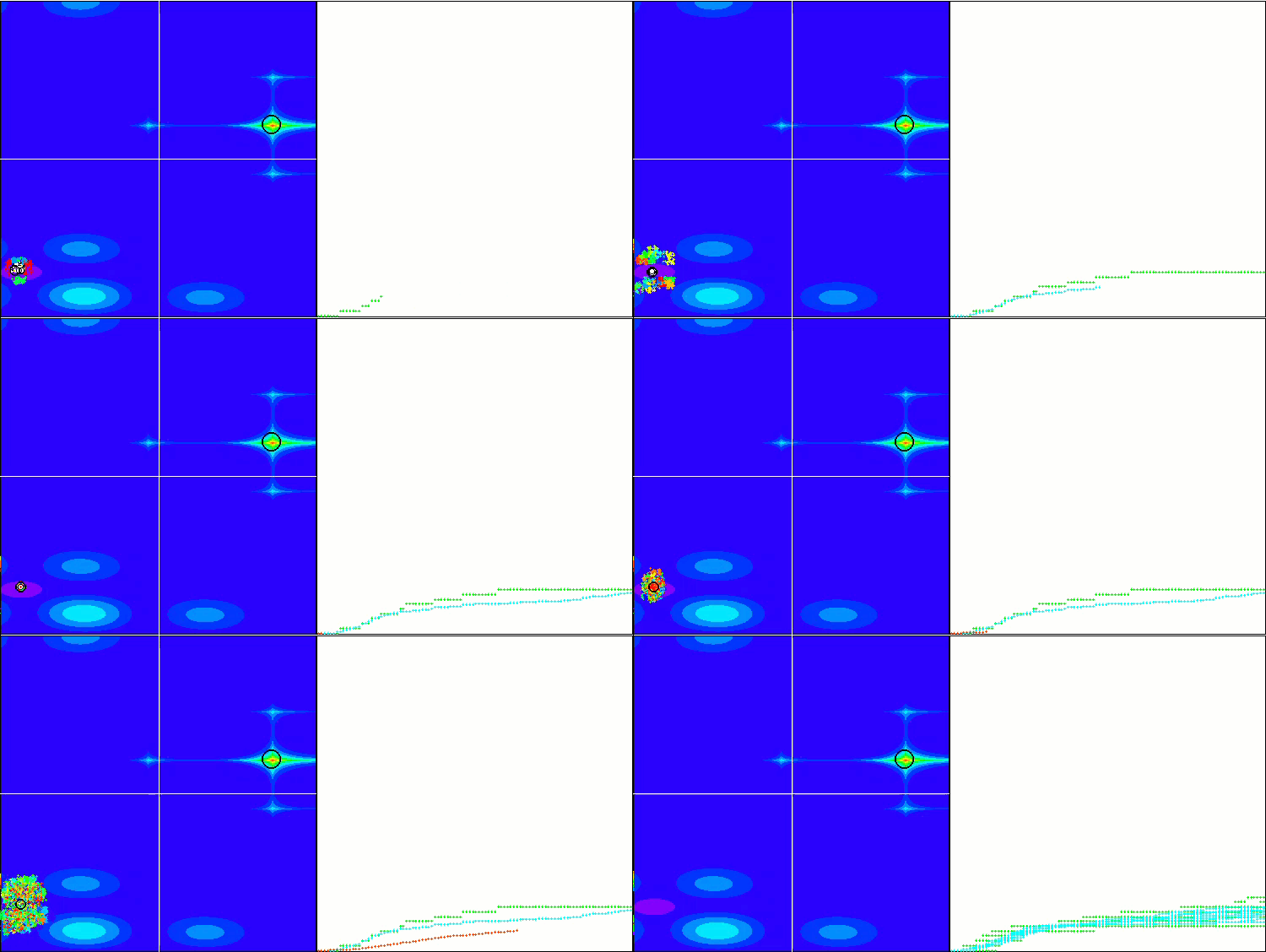
(PO)ES on Megacity

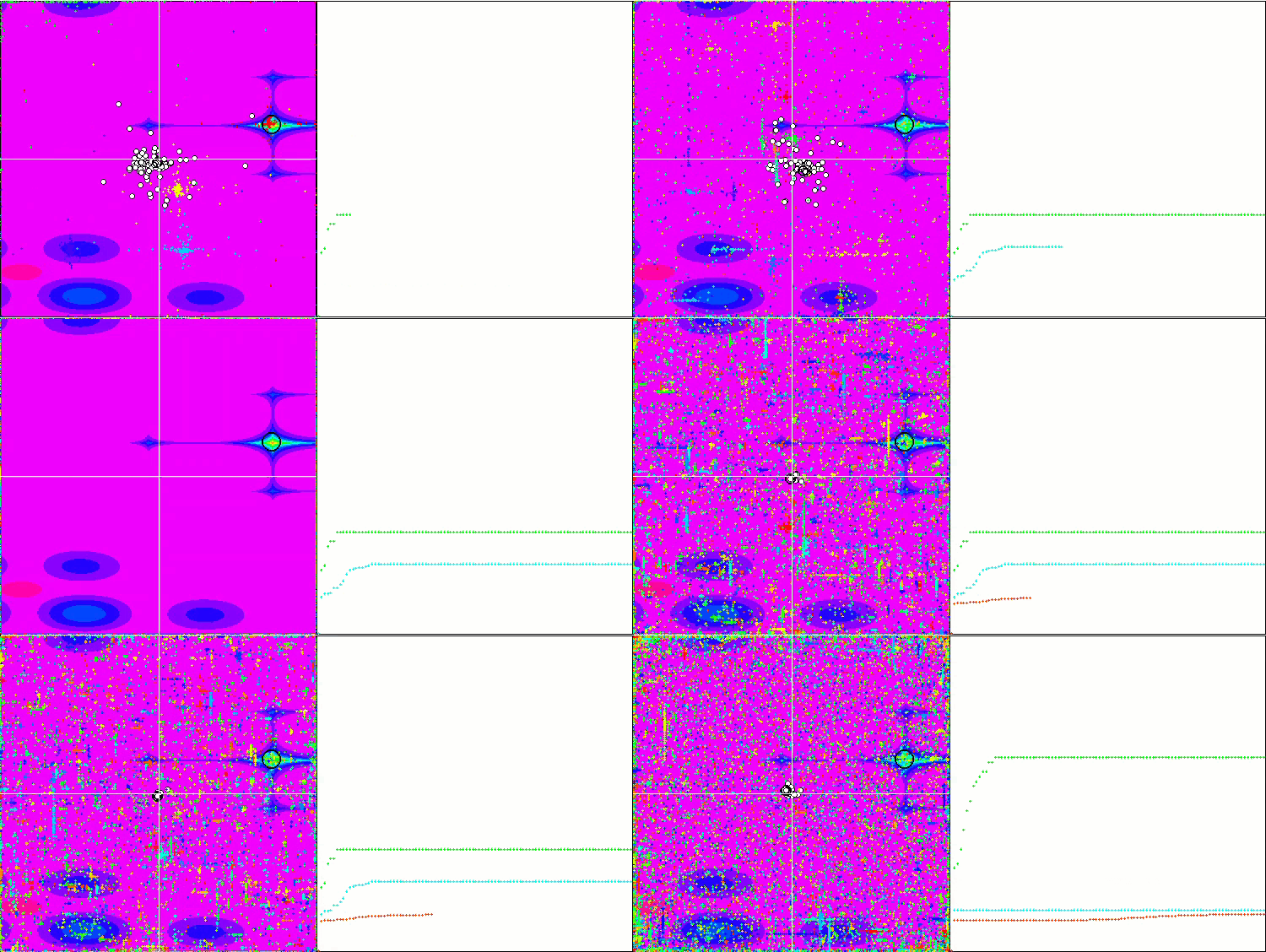
SDOm on Megacity

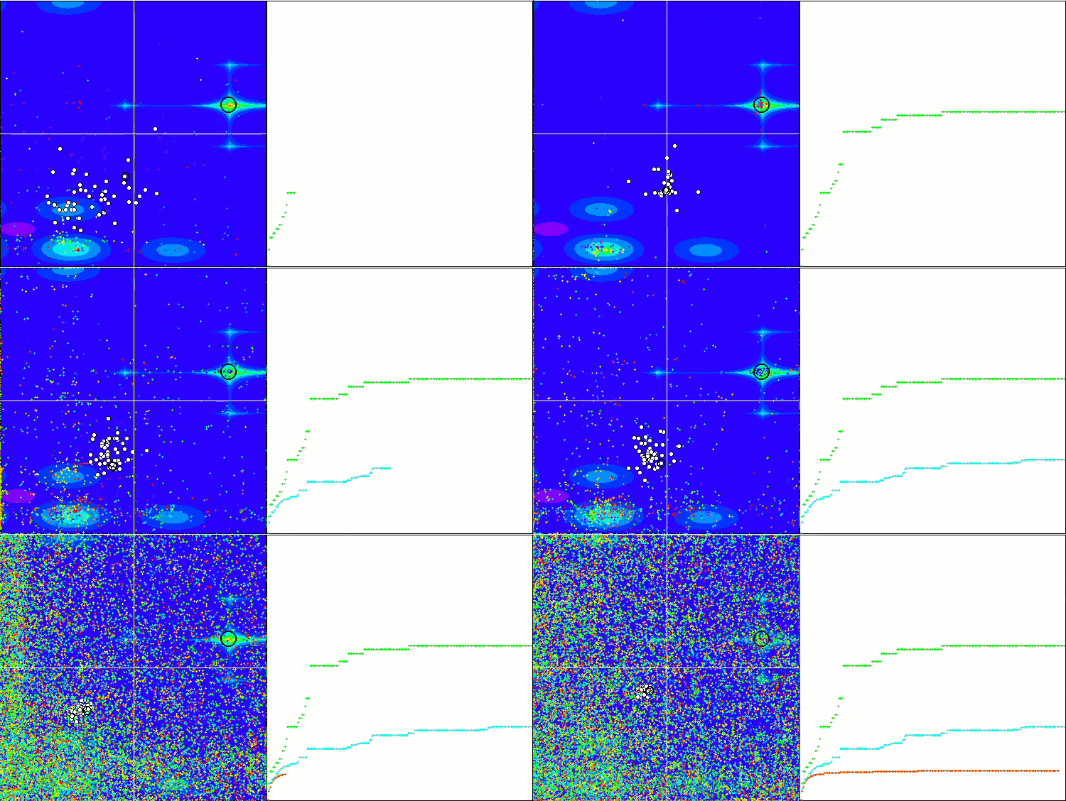
BFO_GA on Megacity

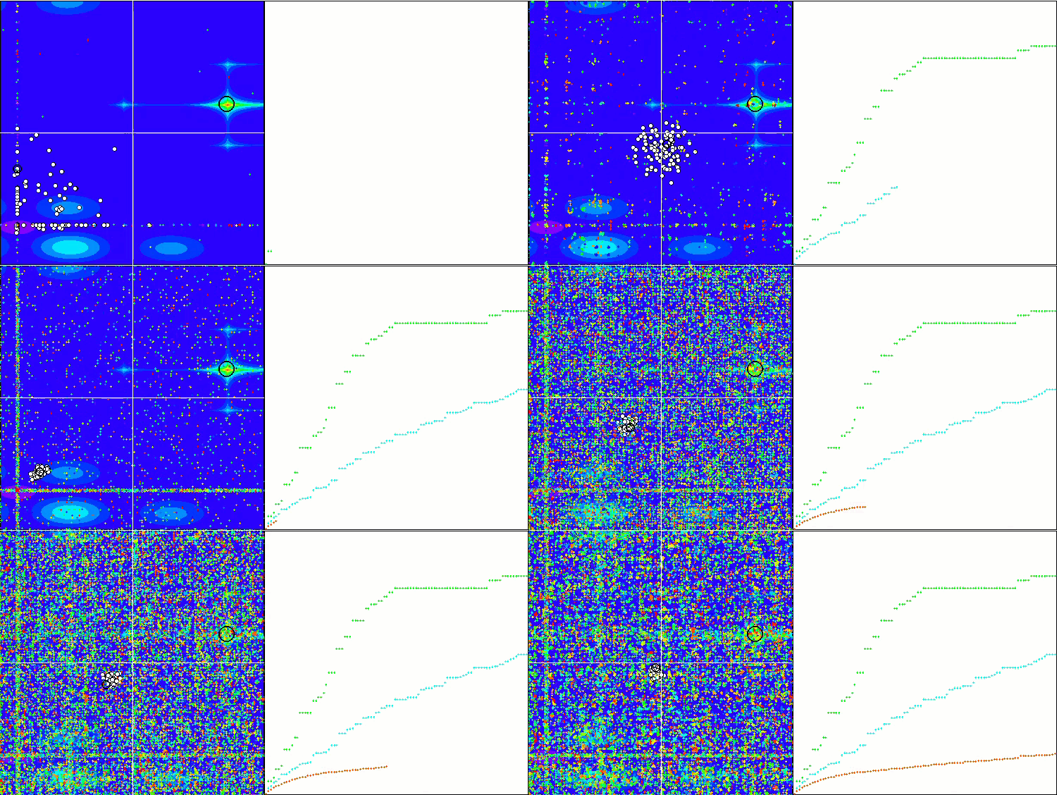
SDSm on Megacity

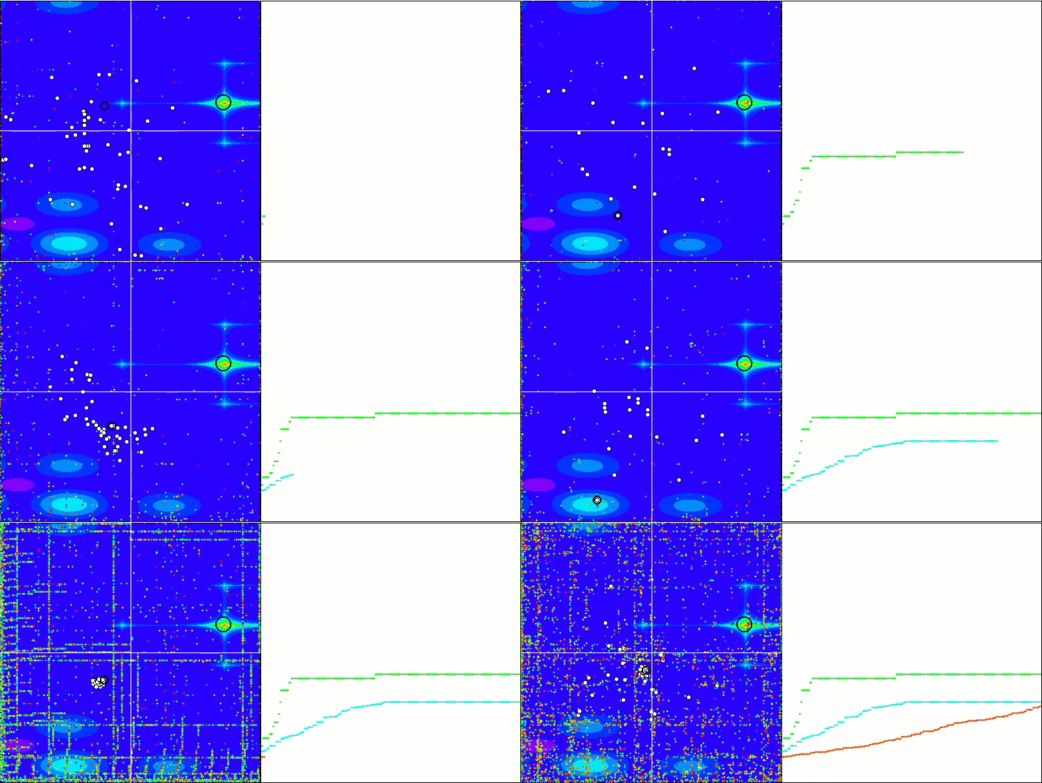
BGA on Megacity

Below is the final comparative table, which shows in detail the work of each algorithm on the test functions.

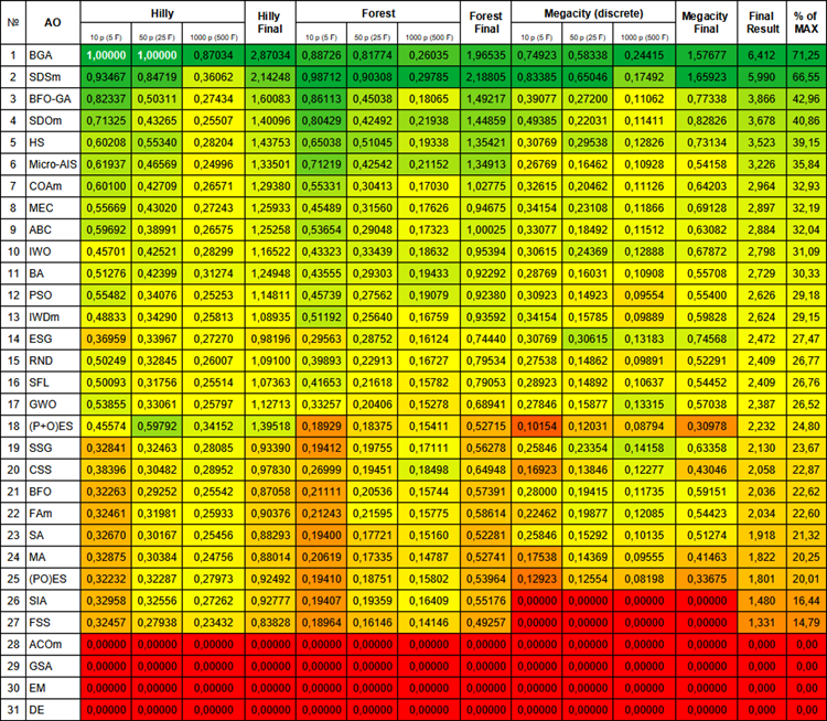
Figure 1. Color gradation of algorithms according to relevant tests Results greater than or equal to 0.99 are highlighted in white

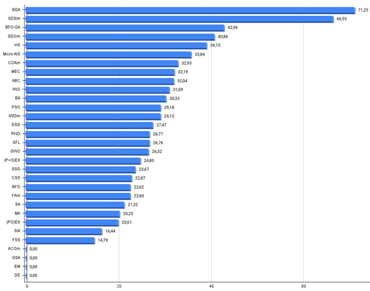
Figure 2. The histogram of algorithm test results (on a scale from 0 to 100, the more the better,

where 100 is the maximum possible theoretical result, the archive features a script for calculating the rating table)

In conclusion, I want to specifically emphasize that all conclusions and judgments for each algorithm were made exclusively within the framework of the experiment.

The entire discussion and analysis of the population optimization algorithms behavior suggest that the success of the algorithms strongly depends on the initial conditions of their application. For some methods, such as DE, EM, GSA, ACOm, tests with an exit from the minimum point of the test function can be so complex that they lead to difficulties at the very start. At the same time, for others, such as (P+O)ES, ESG (which initially occupied the top positions in the ranking, but became outsiders), the efficiency is sharply reduced. On the contrary, deliberately selected initial coordinates can significantly improve the results for such algorithms as PSO, GWO, SFL, BA and ABC. Some algorithms (BFO-GA and SDOm) have even demonstrated outstanding performance with this approach, outperforming random uniform agent initialization.

Other algorithms, such as IWO, HS, SDSm and BGA, have shown universal stability regardless of the starting position of the agents. This special experiment highlighted that although some algorithms performed poorly during the test, they still demonstrated impressive abilities at certain points in the experiment. Some of them successfully explored the space early in the process, while others were able to significantly improve the results in later stages. These unique features of each algorithm can be successfully combined and hybridized, enhancing their positive aspects and reducing their disadvantages, which can ultimately lead to more efficient optimization methods.