Developing a robot in Python and MQL5 (Part 2): Model selection, creation and training, Python custom tester

Brief summary of the previous article

In the previous article, we talked a bit about machine learning, performed data augmentation, developed features for the future model and selected the best of them. Now it is time to move on and create a working machine learning model that will learn from our features and trade (hopefully successfully). To evaluate the model, we will write a custom Python tester that will help us evaluate the performance of the model and the beauty of the test graphs. For more beautiful test graphs and greater model stability, we will also develop a number of classic machine learning features along the way.

Our ultimate goal is to create a working and maximally profitable model for price forecasting and trading. All code will be in Python, with inclusions of the MQL5 library. 

Python version and required modules

I used Python version 3.10.10 in my work.

The code attached below contains several functions for data preprocessing, feature extraction, and training a machine learning model. In particular, it includes:

• The function for feature clustering using Gaussian Mixture Model (GMM) from the sklearn library
• The feature extraction function using Recursive Feature Elimination with Cross-Validation (RFECV) from the sklearn library
• The function for training the XGBoost classifier

To run the code, you need to install the following Python modules:

• pandas
• numpy
• sklearn
• xgboost
• matplotlib
• seaborn
• MetaTrader 5
  
• tqdm
  

You can install them using 'pip' - the Python package installation utility. Here is an example command to install all the required modules:

pip install pandas numpy sklearn xgboost matplotlib seaborn tqdm MetaTrader5

Let's go!

Classification or regression?

This is one of the eternal questions in data forecasting. Classification is better suited for binary problems where a clear yes-no answer is needed. There is also multi-class classification. We will discuss it in future articles of the series as it can significantly strengthen the models.

Regression is suitable for a specific forecast of a certain future value of a continuous series, including a price series. On the one hand, this can be much more convenient, but on the other hand, data labeling for regression, just like labels themselves, is a challenging topic, because there is little we can do other than just take the future price of the asset. 

I personally like classification more because it simplifies working with data labeling. A lot of things can be driven into yes-no conditions, while the multi-class classification can be applied to entire complex manual trading systems like Smart Money. You have already seen the data labeling code in the previous article of the series, and it is clearly suitable for binary classification. That is why we will take this particular model structure.

It remains to decide on the model itself.

Selecting a classification model

We need to select a suitable classification model for our data with the selected features. The choice depends on the number of features, data types, and number of classes.

Popular models are logistic regression for binary classification, random forest for high dimensions and nonlinearities, neural networks for complex problems. The choice is huge. Having tried many things, I came to the conclusion that in today's conditions the most effective is boosting and models based on it. 

I decided to use the cutting-edge XGBoost model - boosting over decision trees with regularization, parallelism, and lots of settings. XGBoost often wins data science competitions due to its high accuracy. This became the main criterion for choosing a model. 

Generating classification model code

The code uses the state-of-the-art XGBoost model - gradient boosting over decision trees. A special feature of XGBoost is the use of second derivatives for optimization, which increases efficiency and accuracy compared to other models. 

The train_xgboost_classifier function receives the data and the number of boosting rounds. It splits data into X features and y labels, creates the XGBClassifier model with hyperparameter tuning and trains it using the fit() method.

The data is divided into train/test, the model is trained on the training data using the function. The model is tested on the remaining data, and the accuracy of predictions is calculated.

The main advantages of XGBoost are combining multiple models into a highly accurate one using gradient boosting and optimizing for second derivatives for efficiency.

We will also need to install the OpenMP runtime library to use it. For Windows, you need to download the Microsoft Visual C++ Redistributable that matches your Python version.

Let's move on to the code itself. At the beginning of the code, we import the xgboost library the following way:

import xgboost as xgb

The rest of the code:

import xgboost as xgb

def train_xgboost_classifier(data, num_boost_rounds=500):
    # Check if data is not empty
    if data.empty:
        raise ValueError("Data should not be empty")
    
    # Check if all required columns are present in the data
    required_columns = ['label', 'labels']
    if not all(column in data.columns for column in required_columns):
        raise ValueError(f"Data is missing required columns: {required_columns}")
    
    # Remove the 'label' column as it is not a feature
    X = data.drop(['label', 'labels'], axis=1)
    y = data['labels']
    
    # Check if all features have numeric data type
    if not all(pd.api.types.is_numeric_dtype(X[column]) for column in X.columns):
        raise ValueError("All features should have numeric data type")
    
    # Create an XGBoostClassifier model
    clf = xgb.XGBClassifier(objective='binary:logistic', max_depth=10, learning_rate=0.3, n_estimators=num_boost_rounds, random_state=1)
    
    # Train the model on the data
    clf.fit(X, y)
    
    # Return the trained model
    return clf

labeled_data_engineered = feature_engineering(labeled_data_clustered, n_features_to_select=20)

# Get all data
raw_data = labeled_data_engineered

# Test the model on all data
train_data = raw_data[raw_data.index <= FORWARD]

# Test the model on all data
test_data = raw_data[raw_data.index >= FORWARD]

# Train the XGBoost model on the filtered data
xgb_clf = train_xgboost_classifier(train_data, num_boost_rounds=100)

# Test the model on all data
test_data = raw_data[raw_data.index >= FORWARD]
X_test = test_data.drop(['label', 'labels'], axis=1)
y_test = test_data['labels']
predicted_labels = xgb_clf.predict(X_test)

# Calculate prediction accuracy
accuracy = (predicted_labels == y_test).mean()
print(f"Prediction accuracy: {accuracy:.2f}")

Let's train the model and see the Accuracy at 52%.

Our classification accuracy is now 53% of profitable labels. Please note that here we are talking about forecasting situations when the price has changed by more than the take profit (200 pips) and has not touched the stop (100 pips) with its tail. In practice, we will have a profit factor of approximately three, which is quite sufficient for profitable trading. The next step is writing a custom tester in Python to analyze the profitability of models in USD (not in points). It is necessary to understand whether the model is making money taking into account the markup, or whether it is draining the funds.

Implementing the function of the custom tester in Python

def test_model(model, X_test, y_test, markup, initial_balance=10000.0, point_cost=0.00001):
    balance = initial_balance
    trades = 0
    profits = []

    # Test the model on the test data
    predicted_labels = model.predict(X_test)
    for i in range(len(predicted_labels) - 48):
        if predicted_labels[i] == 1:
            # Open a long position
            entry_price = X_test.iloc[i]['close']
            exit_price = X_test.iloc[i+48]['close']
            if exit_price > entry_price + markup:
                # Close the long position with profit
                profit = (exit_price - entry_price - markup) / point_cost
                balance += profit
                trades += 1
                profits.append(profit)
            else:
                # Close the long position with loss
                loss = (entry_price - exit_price + markup) / point_cost
                balance -= loss
                trades += 1
                profits.append(-loss)
        elif predicted_labels[i] == 0:
            # Open a short position
            entry_price = X_test.iloc[i]['close']
            exit_price = X_test.iloc[i+48]['close']
            if exit_price < entry_price - markup:
                # Close the short position with profit
                profit = (entry_price - exit_price - markup) / point_cost
                balance += profit
                trades += 1
                profits.append(profit)
            else:
                # Close the short position with loss
                loss = (exit_price - entry_price + markup) / point_cost
                balance -= loss
                trades += 1
                profits.append(-loss)

    # Calculate the cumulative profit or loss
    total_profit = balance - initial_balance

    # Plot the balance change over the number of trades
    plt.plot(range(trades), [balance + sum(profits[:i]) for i in range(trades)])
    plt.title('Balance Change')
    plt.xlabel('Trades')
    plt.ylabel('Balance ($)')
    plt.xticks(range(0, len(X_test), int(len(X_test)/10)), X_test.index[::int(len(X_test)/10)].strftime('%Y-%m-%d'))  # Add dates to the x-axis
    plt.axvline(FORWARD, color='r', linestyle='--')  # Add a vertical line for the FORWARD date
    plt.show()

    # Print the results
    print(f"Cumulative profit or loss: {total_profit:.2f} $")
    print(f"Number of trades: {trades}")

# Get test data
test_data = raw_data[raw_data.index >= FORWARD]
X_test = test_data.drop(['label', 'labels'], axis=1)
y_test = test_data['labels']

# Test the model with markup and target labels
initial_balance = 10000.0
markup = 0.00001
test_model(xgb_clf, X_test, y_test, markup, initial_balance)

The code creates a function to test the machine learning model on test data and analyze its profitability taking into account the markup (this should include losses on spreads and various types of commissions). Swaps are not taken into account, since they are dynamic and depend on key rates. They can be taken into account by simply adding a couple of pips to the markup.

The function receives a model, test data, markup and initial balance. Trading is simulated using the model predictions: long at 1, short at 0. If the profit exceeds the markup, the position is closed and the profit is added to the balance.

Trades and profit/loss from each position is saved. The balance chart is constructed. The accumulated total profit/loss is calculated.

At the end, we obtain test data and remove unnecessary columns. The trained xgb_clf model is tested with the given markup and initial balance. Let's test it!

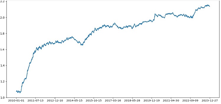
The tester works successfully overall, and we see such a beautiful profitability graph. This is a custom tester for analyzing the profitability of a machine learning trading model taking into account markup and labels.

Implementing cross-validation into the model

We need to use cross-validation to obtain a more reliable assessment of the quality of a machine learning model. Cross-validation allows evaluating a model on multiple data subsets, which helps avoid overfitting and provide a more objective assessment.

In our case, we will use 5-fold cross-validation to evaluate the XGBoost model. To do this, we will use the cross_val_score function from the sklearn library.

Let's change the code of the train_xgboost_classifier function as follows:

def train_xgboost_classifier(data, num_boost_rounds=500):
    # Check that data is not empty
    if data.empty:
        raise ValueError("Data should not be empty")

    # Check that all required columns are present in the data
    required_columns = ['label', 'labels']
    if not all(column in data.columns for column in required_columns):
        raise ValueError(f"Data is missing required columns: {required_columns}")

    # Drop the 'label' column since it is not a feature
    X = data.drop(['label', 'labels'], axis=1)
    y = data['labels']

    # Check that all features have numeric data type
    if not all(pd.api.types.is_numeric_dtype(X[column]) for column in X.columns):
        raise ValueError("All features should have numeric data type")

    # Create XGBoostClassifier model
    clf = xgb.XGBClassifier(objective='binary:logistic', max_depth=10, learning_rate=0.3, n_estimators=num_boost_rounds, random_state=1)

    # Train the model on the data using cross-validation
    scores = cross_val_score(clf, X, y, cv=5)

    # Calculate the mean accuracy of the predictions
    accuracy = scores.mean()

    print(f"Mean prediction accuracy on cross-validation: {accuracy:.2f}")

    # Train the model on the data without cross-validation
    clf.fit(X, y)

    # Return the trained model
    return clf

labeled_data_engineered = feature_engineering(labeled_data_clustered, n_features_to_select=20)

# Get all data
raw_data = labeled_data_engineered

# Train data
train_data = raw_data[raw_data.index <= FORWARD]

# Train the XGBoost model on the filtered data
xgb_clf = train_xgboost_classifier(train_data, num_boost_rounds=100)

# Test data
test_data = raw_data[raw_data.index >= FORWARD]
X_test = test_data.drop(['label', 'labels'], axis=1)
y_test = test_data['labels']
predicted_labels = xgb_clf.predict(X_test)

# Calculate the accuracy of the predictions
accuracy = (predicted_labels == y_test).mean()
print(f"Accuracy: {accuracy:.2f}")

When training the model, the train_xgboost_classifier function will perform 5-fold cross-validation and output the average prediction accuracy. The training will still include the sample up to the FORWARD date.

Cross-validation is only used to evaluate the model, not to train it. Training is performed on all data up to the FORWARD date without cross-validation.

Cross-validation allows for a more reliable and objective assessment of the model quality, which in theory will increase its robustness to new price data. Or not? Let's check and see how the tester works.

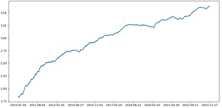
Testing XGBoost with cross-validation on data from 1990-2024 yielded 56% accuracy on the test after 2010. The model showed good robustness to new data on the first try. Accuracy has also improved quite a bit, which is good news.

Optimization of model hyperparameters on a grid

Hyperparameter optimization is an important step in creating a machine learning model to maximize its accuracy and performance. It is similar to optimizing MQL5 EAs, just imagine that instead of an EA you have a machine learning model. Using grid search, you find the parameters that will perform best.

Let's look at grid-based XGBoost hyperparameter optimization using Scikit-learn.

We will use GridSearchCV from Scikit-learn to cross-validate the model across all hyperparameter sets of the grid. The set with the highest average accuracy in cross-validation will be selected.

Optimization code:

from sklearn.model_selection import GridSearchCV

# Define the grid of hyperparameters
param_grid = {
    'max_depth': [3, 5, 7, 10],
    'learning_rate': [0.1, 0.3, 0.5],
    'n_estimators': [100, 500, 1000]
}

# Create XGBoost model
clf = xgb.XGBClassifier(objective='binary:logistic', random_state=1)

# Perform grid search to find the best hyperparameters
grid_search = GridSearchCV(clf, param_grid, cv=5, scoring='accuracy')
grid_search.fit(X_train, y_train)

# Print the best hyperparameters
print("Best hyperparameters:", grid_search.best_params_)

# Print the mean accuracy of the predictions on cross-validation for the best hyperparameters
print("Mean prediction accuracy on cross-validation:", grid_search.best_score_)

Here we define a grid of hyperparameters param_grid, create the XGBoost clf model and search for optimal hyperparameters over the grid using the GridSearchCV method. We then output the best hyperparameters grid_search.best_params_ and the average cross-validation prediction accuracy grid_search.best_score_.

Note that in this code we use cross-validation to optimize hyperparameters. This allows us to obtain a more reliable and objective assessment of the model quality.

After running this code, we get the best hyperparameters for our XGBoost model and the average prediction accuracy on cross-validation. We can then train the model on all the data using the best hyperparameters and test it on new data.

Thus, optimizing the model hyperparameters over a grid is an important task when creating machine learning models. Using the GridSearchCV method from the Scikit-learn library, we can automate this process and find the best hyperparameters for a given model and data.

def train_xgboost_classifier(data, num_boost_rounds=1000):
    # Check that data is not empty
    if data.empty:
        raise ValueError("Data should not be empty")

    # Check that all required columns are present in the data
    required_columns = ['label', 'labels']
    if not all(column in data.columns for column in required_columns):
        raise ValueError(f"Data is missing required columns: {required_columns}")

    # Drop the 'label' column since it is not a feature
    X = data.drop(['label', 'labels'], axis=1)
    y = data['labels']

    # Check that all features have numeric data type
    if not all(pd.api.types.is_numeric_dtype(X[column]) for column in X.columns):
        raise ValueError("All features should have numeric data type")

    # Create XGBoostClassifier model
    clf = xgb.XGBClassifier(objective='binary:logistic', random_state=1)

    # Define hyperparameters for grid search
    param_grid = {
        'max_depth': [3, 5, 7, 10],
        'learning_rate': [0.05, 0.1, 0.2, 0.3, 0.5],
        'n_estimators': [50, 100, 600, 1200, 2000]
    }

    # Train the model on the data using cross-validation and grid search
    grid_search = GridSearchCV(clf, param_grid, cv=5, scoring='accuracy')
    grid_search.fit(X, y)

    # Calculate the mean accuracy of the predictions
    accuracy = grid_search.best_score_

    print(f"Mean prediction accuracy on cross-validation: {accuracy:.2f}")

    # Return the trained model with the best hyperparameters
    return grid_search.best_estimator_

Model ensembling

It is time to make our model even cooler and better! Model ensembling is a powerful approach in machine learning that combines multiple models to improve prediction accuracy. Popular methods include bagging (creating models on different subsamples of data) and boosting (sequentially training models to correct the errors of previous ones).

In our task, we use XGBoost ensemble with bagging and boosting. We create several XGBoosts trained on different subsamples and combine their predictions. We also optimize the hyperparameters of each model with GridSearchCV.

Benefits of ensembling: higher accuracy, reduced variance, improved overall model quality.

The final model training function uses cross-validation, ensembling and grid bagging hyperparameter selection.

def train_xgboost_classifier(data, num_boost_rounds=1000):
    # Check that data is not empty
    if data.empty:
        raise ValueError("Data should not be empty")

    # Check that all required columns are present in the data
    required_columns = ['label', 'labels']
    if not all(column in data.columns for column in required_columns):
        raise ValueError(f"Missing required columns in data: {required_columns}")

    # Remove the 'label' column as it is not a feature
    X = data.drop(['label', 'labels'], axis=1)
    y = data['labels']

    # Check that all features have numeric data type
    if not all(pd.api.types.is_numeric_dtype(X[column]) for column in X.columns):
        raise ValueError("All features should have numeric data type")

    # Create XGBoostClassifier model
    clf = xgb.XGBClassifier(objective='binary:logistic', random_state=1)

    # Define hyperparameters for grid search
    param_grid = {
        'max_depth': [3, 7, 12],
        'learning_rate': [0.1, 0.3, 0.5],
        'n_estimators': [100, 600, 1200]
    }

    # Train the model on the data using cross-validation and hyperparameter tuning
    grid_search = GridSearchCV(clf, param_grid, cv=5, scoring='accuracy')
    grid_search.fit(X, y)

    # Calculate the mean accuracy of the predictions
    accuracy = grid_search.best_score_

    print(f"Mean accuracy on cross-validation: {accuracy:.2f}")

    # Return the trained model
    return grid_search.best_estimator_

labeled_data_engineered = feature_engineering(labeled_data_clustered, n_features_to_select=20)

# Get all data
raw_data = labeled_data_engineered

# Train data
train_data = raw_data[raw_data.index <= FORWARD]

# Test data
test_data = raw_data[raw_data.index <= EXAMWARD]

# Train the XGBoost model on the filtered data
xgb_clf = train_xgboost_classifier(train_data, num_boost_rounds=100)

# Test the model on all data
test_data = raw_data[raw_data.index >= FORWARD]
X_test = test_data.drop(['label', 'labels'], axis=1)
y_test = test_data['labels']
predicted_labels = xgb_clf.predict(X_test)

# Calculate the accuracy of the predictions
accuracy = (predicted_labels == y_test).mean()
print(f"Prediction accuracy: {accuracy:.2f}")

Implement model ensemble through bagging, perform the test and obtain the following test result:

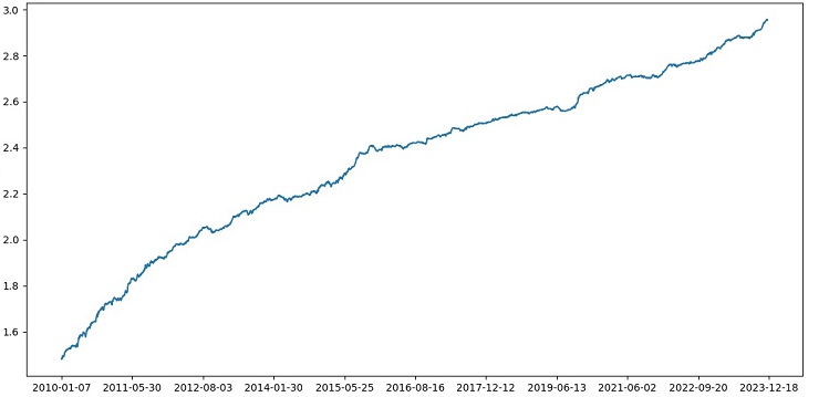
The accuracy of classifying trades with a risk-reward ratio of 1:8 increased to 73%. In other words, ensembling and grid search have given us a huge boost in classification accuracy compared to the previous version of the code. I consider this a more than excellent result, and from the previous charts of the model's performance in the forward section, one can clearly understand how much it has strengthened during the code evolution.   

 

Implementing the examination sample and testing the model robustness

Now I use data after the EXAMWARD date for the test. This allows me to test the model performance on completely new data that was not used to train and test the model. This way I can objectively assess how the model will perform in real conditions.

Testing on an exam sample is an important step in validating a machine learning model. This ensures that the model performs well on new data and gives an idea of its real-world performance. Here we need to correctly determine the sample size and ensure that it is representative.

In my case, I use post-EXAMWARD data to test the model on completely unfamiliar data outside of train and test. This way I get an objective assessment of the model efficiency and readiness for real use.

I conducted training on data from 2000-2010, test on 2010-2019, exam - from 2019. The exam simulates trading in an unknown future.

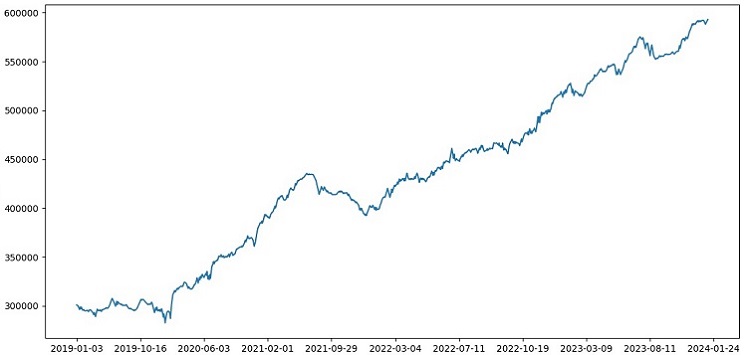
Overall, everything looks good. The accuracy on the exam dropped to 60%, but the main thing is that the model is profitable and quite robust, while having no strong drawdowns. It is pleasing that the model learns the concept of risk/reward - it predicts situations with low risk and high potential profit (we use 1:8 risk-reward).

Conclusion

This concludes the second article in the series on creating a trading robot in Python. At the moment, we have managed to solve the problems of working with data, working with features, the problems of selection and even generation of features, as well as the problem of selecting and training a model. We have also implemented a custom tester that tests the model, and it seems like everything is working out pretty well. By the way, I tried other features, including the simplest ones, trying to simplify the data to no avail. Models with these characteristics drained the account in the tester. This once again confirms that features and data are no less important than the model itself. We can make a good model and apply various improvements and methods, but if the features are useless, then it will also shamelessly drain our deposit on unknown data. On the contrary, with good features, you can get a stable result even on a mediocre model. 

Further developments

In the future, I plan to create a custom version of online trading in the MetaTrader 5 terminal to trade directly through Python to boost convenience. After all, my initial incentive to make a version specifically for Python was the problems with transferring features to MQL5. It is still much faster and more convenient for me to handle features, their selection, data labeling and data augmentation in Python.

I believe that the MQL5 library for Python is unfairly underrated. It is clear that few people use it. It is a powerful solution that can be used to create truly beautiful models that are pleasing to both the eye and the wallet!

I would also like to implement a version that will learn from the market depth historical data of a real exchange - CME or MOEX. This is also a promising endeavor.