William Gann methods (Part III): Does Astrology Work?

Introduction

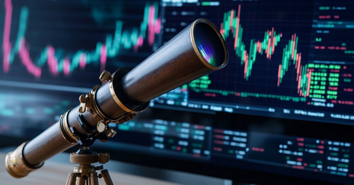
The financial market participants are constantly searching for new and new methods of market analysis and forecasting. Even the most incredible concepts are not left out. One of the non-standard and completely unique approaches is the use of astrology in trading, which was popularized by the famous trader William Gann.

We have already touched upon Gann's tools in our previous articles. Here are the first and second parts. We will now focus on exploring the impact of planetary and stellar positions on world markets.

Let's try to combine the most modern technologies and ancient knowledge. We will use the Python programming language, as well as the MetaTrader 5 platform to find the connection between astronomical phenomena and the movements of the EURUSD pair. We will cover the theoretical part of astrology in finance, and try ourselves in the practical part of developing a forecasting system.

Besides, we will look at collecting and synchronizing astronomical and financial data, create a correlation matrix, and visualize the results. 

Theoretical basis of astrology in finance

I have been interested in this topic for a long time, and today I want to share my thoughts on the influence of astrology on financial markets. This is a really fascinating area, although quite controversial.

The basic idea of financial astrology, as I understand it, is that the movements of the celestial bodies are somehow related to market cycles. This concept has a long and rich history, and was especially popularized by William Gann, a famous trader of the last century.

I have thought a lot about the basic principles of this theory. For example, the idea of cyclicism stating that the movements of stars and planets are cyclical in nature, as are the market movements. In terms of planetary aspects, some believe that certain planetary positions have a strong influence on the markets. And what about the zodiac signs? It is believed that the passage of planets through different zodiac constellations also somehow affects the market.

Lunar cycles and solar activity are worth mentioning as well. I have seen opinions that the phases of the moon are associated with short-term fluctuations in the market, while solar flares are associated with long-term trends. Interesting hypotheses, aren't they?

William Gunn was a real pioneer in this field. He developed a number of tools, such as his famous square of 9, based on astronomy, geometry and number sequences. His works still cause heated debate.

Of course, it cannot be ignored that the scientific community as a whole is skeptical about astrology. In many countries, it is officially recognized as pseudoscience. And frankly speaking, there is no strict evidence yet of the efficiency of astrological methods in finance. Often, certain observed correlations turn out to be simply the result of cognitive biases.

Despite this, there are many traders who ardently defend the ideas of financial astrology.

That is why I decided to do my own research. I would like to try to give an objective assessment of the influence of astrology on financial markets using statistical methods and big data. Who knows, maybe we will discover something interesting. Either way, it will be a fascinating journey into the world where stars and stock charts intersect.

Overview of applied Python libraries

I will need a whole arsenal of Python libraries. 

To start with, I decided to use the Skyfield package to obtain astronomical data. I spent a long time choosing the right tool, and Skyfield impressed me with its precision. With its help, I will be able to collect information about the positions of celestial bodies and the phases of the moon with very high accuracy in decimal places - everything that is needed for my datasets.

As for market data, my choice fell on the official MetaTrader 5 library for Python. It will allow downloading historical data on currency pairs and even open trades if necessary.

Pandas will become our faithful companion in working with data. I have used this library a lot in the past and it is simply indispensable for working with time series. I will use it for pre-processing and synchronization of all collected data.

For statistical analysis, I settled on the SciPy library. Its wide functionality is impressive, especially the tools for correlation and regression analysis. I hope they will help me find interesting patterns.

To visualize the results, I decided to use my good old friends - Matplotlib and Seaborn. I love these libraries for their flexibility in creating graphs. I am sure they will help visualize all the findings.

The whole set is assembled. It is like assembling a powerful PC from excellent components. We now have everything we need to conduct a comprehensive study of the influence of astrological factors on financial markets. I can't wait to dive into the data and start testing my hypotheses!

Collecting astronomical data

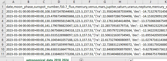
import pandas as pd
import numpy as np
from skyfield.api import load, wgs84, utc
from skyfield.data import mpc
from datetime import datetime, timedelta
import requests

# Loading planet ephemerides
planets = load('de421.bsp')
earth = planets['earth']
ts = load.timescale()

def get_planet_positions(date):
    t = ts.from_datetime(date.replace(tzinfo=utc))
    planet_positions = {}
    planet_ids = {
        'mercury': 'MERCURY BARYCENTER',
        'venus': 'VENUS BARYCENTER',
        'mars': 'MARS BARYCENTER',
        'jupiter': 'JUPITER BARYCENTER',
        'saturn': 'SATURN BARYCENTER',
        'uranus': 'URANUS BARYCENTER',
        'neptune': 'NEPTUNE BARYCENTER'
    }
    for planet, planet_id in planet_ids.items():
        planet_obj = planets[planet_id]
        astrometric = earth.at(t).observe(planet_obj)
        ra, dec, _ = astrometric.radec()
        planet_positions[planet] = {'ra': ra.hours, 'dec': dec.degrees}
    return planet_positions

def get_moon_phase(date):
    t = ts.from_datetime(date.replace(tzinfo=utc))
    eph = load('de421.bsp')
    moon, sun, earth = eph['moon'], eph['sun'], eph['earth']
    
    e = earth.at(t)
    _, m, _ = e.observe(moon).apparent().ecliptic_latlon()
    _, s, _ = e.observe(sun).apparent().ecliptic_latlon()
    
    phase = (m.degrees - s.degrees) % 360
    return phase

def get_solar_activity(date):
    # Get solar activity data from NOAA API
    url = f"https://services.swpc.noaa.gov/json/solar-cycle/observed-solar-cycle-indices.json"
    response = requests.get(url)
    data = response.json()
    
    # Convert date to 'YYYY-MM' format
    target_date = date.strftime("%Y-%m")
    
    # Find the closest date in the data
    closest_data = min(data, key=lambda x: abs(datetime.strptime(x['time-tag'], "%Y-%m") - datetime.strptime(target_date, "%Y-%m")))
    
    return {
        'sunspot_number': closest_data.get('ssn', None),
        'f10.7_flux': closest_data.get('f10.7', None)
    }

def calculate_aspects(positions):
    aspects = {}
    planets = list(positions.keys())
    for i in range(len(planets)):
        for j in range(i+1, len(planets)):
            planet1 = planets[i]
            planet2 = planets[j]
            ra1 = positions[planet1]['ra']
            ra2 = positions[planet2]['ra']
            angle = abs(ra1 - ra2) % 24
            angle = min(angle, 24 - angle) * 15  # Convert to degrees
            
            if abs(angle - 0) <= 10 or abs(angle - 180) <= 10:
                aspects[f"{planet1}_{planet2}"] = "conjunction" if abs(angle - 0) <= 10 else "opposition"
            elif abs(angle - 90) <= 10:
                aspects[f"{planet1}_{planet2}"] = "square"
            elif abs(angle - 120) <= 10:
                aspects[f"{planet1}_{planet2}"] = "trine"
    
    return aspects

start_date = datetime(2024, 4, 1, tzinfo=utc)
end_date = datetime(2024, 5, 31, tzinfo=utc)
current_date = start_date
astronomical_data = []

while current_date <= end_date:
    planet_positions = get_planet_positions(current_date)
    moon_phase = get_moon_phase(current_date)
    try:
        solar_activity = get_solar_activity(current_date)
    except Exception as e:
        print(f"Error getting solar activity for {current_date}: {e}")
        solar_activity = {'sunspot_number': None, 'f10.7_flux': None}
    aspects = calculate_aspects(planet_positions)
    
    data = {
        'date': current_date,
        'moon_phase': moon_phase,
        'sunspot_number': solar_activity.get('sunspot_number'),
        'f10.7_flux': solar_activity.get('f10.7_flux'),
        **planet_positions,
        **aspects
    }
    astronomical_data.append(data)
    
    current_date += timedelta(days=1)
    print(f"Processed: {current_date}")

# Convert data to DataFrame
df = pd.DataFrame(astronomical_data)

# Save data to CSV file
df.to_csv('astronomical_data_2018_2024.csv', index=False)
print("Data saved to astronomical_data_2018_2024.csv")

This Python code collects astronomical data that we will use in the future for market analysis.

The code uses the period from January 1, 2018 to May 31, 2024, and collects a range of data such as:

• Positions of the planets - Venus, Mercury, Mars, Jupiter, Saturn, Uranus and Neptune
• Lunar phases
• Solar activity
• Planet aspects (how planets are aligned in relation to each other)

The script includes library imports, the main loop, and saving data in Excel format. The code uses the already mentioned Skyfield library to calculate planet positions, Pandas for data, and requests to obtain solar activity data.

The noteworthy functions include get_planet_positions() for getting the positions of the planets (right ascension and declination), get_moon_phase() for finding the current lunar phase, get_solar_activity() for direct delivery of solar activity data from the NOAA API, and calculate_aspects() for calculating aspects – the positions of the planets in relation to each other.

We go through each day as part of the cycle and collect all the data. As a result, we save everything in one Excel file for future use. 

Getting financial data via MetaTrader 5

To get financial data, we will use the MetaTrader 5 library for Python. The library will allow us to download financial data directly from the broker and receive time series of prices for any instrument. Here is our code for loading historical data: 

import MetaTrader5 as mt5
import pandas as pd
from datetime import datetime

# Connect to MetaTrader5
if not mt5.initialize():
    print("initialize() failed")
    mt5.shutdown()

# Set query parameters
symbol = "EURUSD"
timeframe = mt5.TIMEFRAME_D1
start_date = datetime(2018, 1, 1)
end_date = datetime(2024, 12, 31)

# Request historical data
rates = mt5.copy_rates_range(symbol, timeframe, start_date, end_date)

# Convert data to DataFrame
df = pd.DataFrame(rates)
df['time'] = pd.to_datetime(df['time'], unit='s')

# Save data to CSV file
df.to_csv(f'{symbol}_data.csv', index=False)

# Terminate the connection to MetaTrader5
mt5.shutdown()

The script connects to the trading terminal, receives data on EURUSD D1, then creates a dataframe and saves it in a single CSV file. 

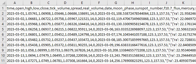
Synchronizing astronomical and financial data

So we have data on astronomy, we also have data on EURUSD. Now we have to synchronize them. Let's combine the data by dates so that a single dataset contains all the necessary information, both financial and astronomical.

import pandas as pd

# Load data
astro_data = pd.read_csv('astronomical_data_2018_2024.csv')
financial_data = pd.read_csv('EURUSD_data.csv')

# Convert date columns to datetime
astro_data['date'] = pd.to_datetime(astro_data['date'])
financial_data['time'] = pd.to_datetime(financial_data['time'])

# Merge data
merged_data = pd.merge(financial_data, astro_data, left_on='time', right_on='date', how='inner')

# Save merged data
merged_data.to_csv('merged_astro_financial_data.csv', index=False)

The script loads all saved data, formats date columns into datetime format, and combines datasets by date. As a result, we get a CSV file that contains all the data we need for future analysis.

Statistical analysis of correlations

Let's move on. We have a common set, a common dataset, and it is time to find out if there are any relationships in the data between astronomy nd market movements. We will use the corr() functions from the pandas library. Besides, we will combine both of our codes into one.

Here is the final script:

import pandas as pd
import numpy as np
from skyfield.api import load, wgs84, utc
from skyfield.data import mpc
from datetime import datetime, timedelta
import requests
import MetaTrader5 as mt5
import seaborn as sns
import matplotlib.pyplot as plt

# Part 1: Collecting astronomical data

# Loading planetary ephemerides
planets = load('de421.bsp')
earth = planets['earth']
ts = load.timescale()

def get_planet_positions(date):
    t = ts.from_datetime(date.replace(tzinfo=utc))
    planet_positions = {}
    planet_ids = {
        'mercury': 'MERCURY BARYCENTER',
        'venus': 'VENUS BARYCENTER',
        'mars': 'MARS BARYCENTER',
        'jupiter': 'JUPITER BARYCENTER',
        'saturn': 'SATURN BARYCENTER',
        'uranus': 'URANUS BARYCENTER',
        'neptune': 'NEPTUNE BARYCENTER'
    }
    for planet, planet_id in planet_ids.items():
        planet_obj = planets[planet_id]
        astrometric = earth.at(t).observe(planet_obj)
        ra, dec, _ = astrometric.radec()
        planet_positions[planet] = {'ra': ra.hours, 'dec': dec.degrees}
    return planet_positions

def get_moon_phase(date):
    t = ts.from_datetime(date.replace(tzinfo=utc))
    eph = load('de421.bsp')
    moon, sun, earth = eph['moon'], eph['sun'], eph['earth']

    e = earth.at(t)
    _, m, _ = e.observe(moon).apparent().ecliptic_latlon()
    _, s, _ = e.observe(sun).apparent().ecliptic_latlon()

    phase = (m.degrees - s.degrees) % 360
    return phase

def get_solar_activity(date):
    url = f"https://services.swpc.noaa.gov/json/solar-cycle/observed-solar-cycle-indices.json"
    response = requests.get(url)
    data = response.json()

    target_date = date.strftime("%Y-%m")

    closest_data = min(data, key=lambda x: abs(datetime.strptime(x['time-tag'], "%Y-%m") - datetime.strptime(target_date, "%Y-%m")))

    return {
        'sunspot_number': closest_data.get('ssn', None),
        'f10.7_flux': closest_data.get('f10.7', None)
    }

def calculate_aspects(positions):
    aspects = {}
    planets = list(positions.keys())
    for i in range(len(planets)):
        for j in range(i+1, len(planets)):
            planet1 = planets[i]
            planet2 = planets[j]
            ra1 = positions[planet1]['ra']
            ra2 = positions[planet2]['ra']
            angle = abs(ra1 - ra2) % 24
            angle = min(angle, 24 - angle) * 15  # Convert to degrees

            if abs(angle - 0) <= 10 or abs(angle - 180) <= 10:
                aspects[f"{planet1}_{planet2}"] = "conjunction" if abs(angle - 0) <= 10 else "opposition"
            elif abs(angle - 90) <= 10:
                aspects[f"{planet1}_{planet2}"] = "square"
            elif abs(angle - 120) <= 10:
                aspects[f"{planet1}_{planet2}"] = "trine"

    return aspects

# Collecting astronomical data
start_date = datetime(2024, 3, 1, tzinfo=utc)
end_date = datetime(2024, 7, 30, tzinfo=utc)
current_date = start_date
astronomical_data = []

while current_date <= end_date:
    planet_positions = get_planet_positions(current_date)
    moon_phase = get_moon_phase(current_date)
    try:
        solar_activity = get_solar_activity(current_date)
    except Exception as e:
        print(f"Error getting solar activity for {current_date}: {e}")
        solar_activity = {'sunspot_number': None, 'f10.7_flux': None}
    aspects = calculate_aspects(planet_positions)

    data = {
        'date': current_date,
        'moon_phase': moon_phase,
        'sunspot_number': solar_activity.get('sunspot_number'),
        'f10.7_flux': solar_activity.get('f10.7_flux'),
        **planet_positions,
        **aspects
    }
    astronomical_data.append(data)

    current_date += timedelta(days=1)
    print(f"Processed: {current_date}")

# Convert data to DataFrame and save
astro_df = pd.DataFrame(astronomical_data)
astro_df.to_csv('astronomical_data_2018_2024.csv', index=False)
print("Astronomical data saved to astronomical_data_2018_2024.csv")

# Part 2: Retrieving financial data via MetaTrader5

# Initialize connection to MetaTrader5
if not mt5.initialize():
    print("initialize() failed")
    mt5.shutdown()

# Set request parameters
symbol = "EURUSD"
timeframe = mt5.TIMEFRAME_D1
start_date = datetime(2024, 3, 1)
end_date = datetime(2024, 7, 30)

# Request historical data
rates = mt5.copy_rates_range(symbol, timeframe, start_date, end_date)

# Convert data to DataFrame
financial_df = pd.DataFrame(rates)
financial_df['time'] = pd.to_datetime(financial_df['time'], unit='s')

# Save financial data
financial_df.to_csv(f'{symbol}_data.csv', index=False)
print(f"Financial data saved to {symbol}_data.csv")

# Shutdown MetaTrader5 connection
mt5.shutdown()

# Part 3: Synchronizing astronomical and financial data

# Load data
astro_df = pd.read_csv('astronomical_data_2018_2024.csv')
financial_df = pd.read_csv('EURUSD_data.csv')

# Convert date columns to datetime
astro_df['date'] = pd.to_datetime(astro_df['date']).dt.tz_localize(None)
financial_df['time'] = pd.to_datetime(financial_df['time'])

# Merge data
merged_data = pd.merge(financial_df, astro_df, left_on='time', right_on='date', how='inner')

# Save merged data
merged_data.to_csv('merged_astro_financial_data.csv', index=False)
print("Merged data saved to merged_astro_financial_data.csv")

# Part 4: Statistical analysis of correlations

# Select numeric columns for correlation analysis
numeric_columns = merged_data.select_dtypes(include=[np.number]).columns

# Create lags for astronomical data
for col in numeric_columns:
    if col not in ['open', 'high', 'low', 'close', 'tick_volume', 'spread', 'real_volume']:
        for lag in range(1, 6):  # Create lags from 1 to 5
            merged_data[f'{col}_lag{lag}'] = merged_data[col].shift(lag)

# Update list of numeric columns
numeric_columns = merged_data.select_dtypes(include=[np.number]).columns

# Calculate correlation matrix
correlation_matrix = merged_data[numeric_columns].corr()

# Create heatmap of correlations
plt.figure(figsize=(20, 16))
sns.heatmap(correlation_matrix, annot=False, cmap='coolwarm', vmin=-1, vmax=1, center=0)
plt.title('Correlation Matrix of Astronomical Factors (with Lags) and EURUSD Prices')
plt.tight_layout()
plt.savefig('correlation_heatmap_with_lags.png')
plt.close()

# Output the most significant correlations with the closing price
significant_correlations = correlation_matrix['close'].sort_values(key=abs, ascending=False)
print("Most significant correlations with the closing price:")
print(significant_correlations)

# Create a separate correlation matrix for astronomical data with lags and the current price
astro_columns = [col for col in numeric_columns if col not in ['open', 'high', 'low', 'tick_volume', 'spread', 'real_volume']]
astro_columns.append('close')  # Add the current closing price
astro_correlation_matrix = merged_data[astro_columns].corr()

# Create heatmap of correlations for astronomical data with lags and the current price
import seaborn as sns
import matplotlib.pyplot as plt

# Increase the header and axis label font
plt.figure(figsize=(18, 14))
sns.heatmap(astro_correlation_matrix, annot=False, cmap='coolwarm', vmin=-1, vmax=1, center=0, cbar_kws={'label': 'Correlation'})
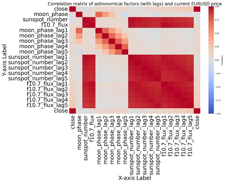
plt.title('Correlation matrix of astronomical factors (with lags) and current EURUSD price', fontsize=24)
plt.xlabel('X-axis Label', fontsize=30)
plt.ylabel('Y-axis Label', fontsize=30)
plt.xticks(fontsize=30)
plt.yticks(fontsize=30)
plt.tight_layout()
plt.savefig('astro_correlation_heatmap_with_lags.png')
plt.close()

print("Analysis completed. Results saved in CSV and PNG files.")

This script displays a map of the correlations between all the numbers in the data set, and also a matrix of all the correlations in heatmap format, as well as produces a list of the most significant correlations with close prices.

The presence or absence of a correlation does not imply the presence or absence of a causal relationship. Even if we found strong correlations between astronomical data and price movements, this would not mean that one factor determines the other, and vice versa. New research is needed, since the correlation map is only the most basic thing.

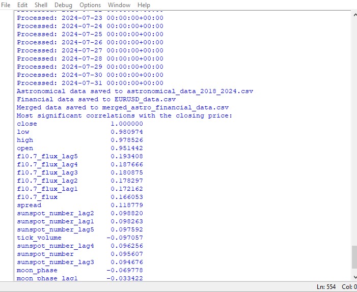
If we get closer to the topic, we are unable to find any significant correlation in the data. There are no clear correlations among past astronomy data with market indicators.

Machine learning to the rescue

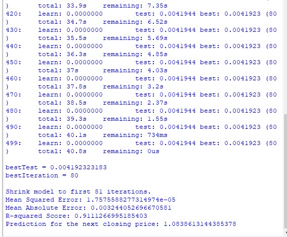
I thought about what to do next and decided to apply a machine learning model. I made two scripts using the CatBoost library that try to predict future prices using data from the dataset as features. Here is the first of the models - a regression one: 

import pandas as pd
import numpy as np
from catboost import CatBoostRegressor
from sklearn.model_selection import train_test_split
from sklearn.metrics import mean_squared_error, mean_absolute_error, r2_score
import matplotlib.pyplot as plt
from sklearn.preprocessing import LabelEncoder

# Loading data
data = pd.read_csv('merged_astro_financial_data.csv')

# Converting date to datetime
data['date'] = pd.to_datetime(data['date'])

# Creating lags for financial data
for col in ['open', 'high', 'low', 'close']:
    for lag in range(1, 6):  # Creating lags from 1 to 5
        data[f'{col}_lag{lag}'] = data[col].shift(lag)

# Creating lags for astronomical data
astro_cols = ['mercury', 'venus', 'mars', 'jupiter', 'saturn', 'uranus', 'neptune']
for col in astro_cols:
    data[f'{col}_ra'] = data[col].apply(lambda x: eval(x)['ra'] if pd.notna(x) else np.nan)
    data[f'{col}_dec'] = data[col].apply(lambda x: eval(x)['dec'] if pd.notna(x) else np.nan)
    for lag in range(1, 6):  # Lags from 1 to 5
        data[f'{col}_ra_lag{lag}'] = data[f'{col}_ra'].shift(lag)
        data[f'{col}_dec_lag{lag}'] = data[f'{col}_dec'].shift(lag)
    data.drop(columns=[col, f'{col}_ra', f'{col}_dec'], inplace=True)

# Converting aspects to numerical features
aspect_cols = ['mercury_saturn', 'venus_mars', 'venus_jupiter', 'venus_uranus', 
               'mars_jupiter', 'mars_uranus', 'jupiter_uranus', 'mercury_neptune', 
               'venus_saturn', 'venus_neptune', 'mars_saturn', 'mercury_venus', 
               'mars_neptune', 'mercury_uranus', 'saturn_neptune', 'mercury_jupiter', 
               'mercury_mars', 'jupiter_saturn']

# Using LabelEncoder for encoding aspects
label_encoders = {}
for col in aspect_cols:
    label_encoders[col] = LabelEncoder()
    data[col] = label_encoders[col].fit_transform(data[col].astype(str))

# Filling missing values with mean values for numeric columns
numeric_cols = data.select_dtypes(include=[np.number]).columns
data[numeric_cols] = data[numeric_cols].fillna(data[numeric_cols].mean())

# Removing rows with missing values
data = data.dropna()

# Preparing features and target variable
features = [col for col in data.columns if col not in ['date', 'time', 'close']]
X = data[features]
y = data['close']

# Splitting data into training and testing sets
X_train, X_test, y_train, y_test = train_test_split(X, y, test_size=0.3, random_state=1)

# Creating and training the CatBoost model
model = CatBoostRegressor(iterations=500, learning_rate=0.1, depth=9, random_state=1)
model.fit(X_train, y_train, eval_set=(X_test, y_test), early_stopping_rounds=200, verbose=100)

# Evaluating the model
y_pred = model.predict(X_test)
mse = mean_squared_error(y_test, y_pred)
mae = mean_absolute_error(y_test, y_pred)
r2 = r2_score(y_test, y_pred)
print(f"Mean Squared Error: {mse}")
print(f"Mean Absolute Error: {mae}")
print(f"R-squared Score: {r2}")

# Visualizing feature importance
feature_importance = model.feature_importances_
feature_names = X.columns
sorted_idx = np.argsort(feature_importance)
pos = np.arange(sorted_idx.shape[0]) + 0.5
plt.figure(figsize=(12, 6))
plt.barh(pos, feature_importance[sorted_idx], align='center')
plt.yticks(pos, np.array(feature_names)[sorted_idx])
plt.xlabel('Feature Importance')
plt.title('Feature Importance')
plt.show()

# Predicting the next value
def predict_next():
    # Selecting the last row of data
    last_data = data.iloc[-1]
    input_features = last_data[features].values.reshape(1, -1)
    # Prediction
    prediction = model.predict(input_features)
    print(f"Prediction for the next closing price: {prediction[0]}")

# Example of using the function to predict the next value
predict_next()

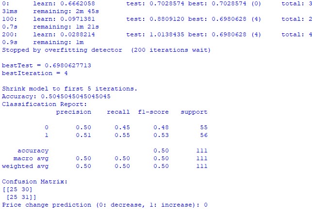
The second model is classification:

import pandas as pd
import numpy as np
from skyfield.api import load, utc
from datetime import datetime, timedelta
import requests
import MetaTrader5 as mt5
import seaborn as sns
import matplotlib.pyplot as plt
from catboost import CatBoostClassifier
from sklearn.model_selection import train_test_split
from sklearn.metrics import accuracy_score, classification_report, confusion_matrix
from sklearn.preprocessing import LabelEncoder

# Part 1: Collecting astronomical data

planets = load('de421.bsp')
earth = planets['earth']
ts = load.timescale()

def get_planet_positions(date):
    t = ts.from_datetime(date.replace(tzinfo=utc))
    planet_positions = {}
    planet_ids = {
        'mercury': 'MERCURY BARYCENTER',
        'venus': 'VENUS BARYCENTER',
        'mars': 'MARS BARYCENTER',
        'jupiter': 'JUPITER BARYCENTER',
        'saturn': 'SATURN BARYCENTER',
        'uranus': 'URANUS BARYCENTER',
        'neptune': 'NEPTUNE BARYCENTER'
    }
    for planet, planet_id in planet_ids.items():
        planet_obj = planets[planet_id]
        astrometric = earth.at(t).observe(planet_obj)
        ra, dec, _ = astrometric.radec()
        planet_positions[planet] = {'ra': ra.hours, 'dec': dec.degrees}
    return planet_positions

def get_moon_phase(date):
    t = ts.from_datetime(date.replace(tzinfo=utc))
    eph = load('de421.bsp')
    moon, sun, earth = eph['moon'], eph['sun'], eph['earth']
    
    e = earth.at(t)
    _, m, _ = e.observe(moon).apparent().ecliptic_latlon()
    _, s, _ = e.observe(sun).apparent().ecliptic_latlon()
    
    phase = (m.degrees - s.degrees) % 360
    return phase

def get_solar_activity(date):
    url = f"https://services.swpc.noaa.gov/json/solar-cycle/observed-solar-cycle-indices.json"
    response = requests.get(url)
    data = response.json()
    
    target_date = date.strftime("%Y-%m")
    
    closest_data = min(data, key=lambda x: abs(datetime.strptime(x['time-tag'], "%Y-%m") - datetime.strptime(target_date, "%Y-%m")))
    
    return {
        'sunspot_number': closest_data.get('ssn', None),
        'f10.7_flux': closest_data.get('f10.7', None)
    }

def calculate_aspects(positions):
    aspects = {}
    planets = list(positions.keys())
    for i in range(len(planets)):
        for j in range(i+1, len(planets)):
            planet1 = planets[i]
            planet2 = planets[j]
            ra1 = positions[planet1]['ra']
            ra2 = positions[planet2]['ra']
            angle = abs(ra1 - ra2) % 24
            angle = min(angle, 24 - angle) * 15  # Convert to degrees
            
            if abs(angle - 0) <= 10 or abs(angle - 180) <= 10:
                aspects[f"{planet1}_{planet2}"] = "conjunction" if abs(angle - 0) <= 10 else "opposition"
            elif abs(angle - 90) <= 10:
                aspects[f"{planet1}_{planet2}"] = "square"
            elif abs(angle - 120) <= 10:
                aspects[f"{planet1}_{planet2}"] = "trine"
    
    return aspects

# Part 2: Obtaining financial data through MetaTrader5

def get_financial_data(symbol, start_date, end_date):
    if not mt5.initialize():
        print("initialize() failed")
        mt5.shutdown()
        return None

    timeframe = mt5.TIMEFRAME_D1

    rates = mt5.copy_rates_range(symbol, timeframe, start_date, end_date)
    mt5.shutdown()

    financial_df = pd.DataFrame(rates)
    financial_df['time'] = pd.to_datetime(financial_df['time'], unit='s')
    return financial_df

# Part 3: Synchronizing astronomical and financial data

def sync_data(astro_df, financial_df):
    astro_df['date'] = pd.to_datetime(astro_df['date']).dt.tz_localize(None)
    financial_df['time'] = pd.to_datetime(financial_df['time'])
    merged_data = pd.merge(financial_df, astro_df, left_on='time', right_on='date', how='inner')
    return merged_data

# Part 4: Training the model and making predictions

def train_and_predict(merged_data):
    # Converting aspects to numerical features
    aspect_cols = [col for col in merged_data.columns if '_' in col and col not in ['date', 'time']]
    label_encoders = {}
    for col in aspect_cols:
        label_encoders[col] = LabelEncoder()
        merged_data[col] = label_encoders[col].fit_transform(merged_data[col].astype(str))
    
    # Creating lags for financial data
    for col in ['open', 'high', 'low', 'close']:
        for lag in range(1, 6):
            merged_data[f'{col}_lag{lag}'] = merged_data[col].shift(lag)
    
    # Creating lags for astronomical data
    astro_cols = ['mercury', 'venus', 'mars', 'jupiter', 'saturn', 'uranus', 'neptune']
    for col in astro_cols:
        merged_data[f'{col}_ra'] = merged_data[col].apply(lambda x: eval(x)['ra'] if pd.notna(x) else np.nan)
        merged_data[f'{col}_dec'] = merged_data[col].apply(lambda x: eval(x)['dec'] if pd.notna(x) else np.nan)
        for lag in range(1, 6):
            merged_data[f'{col}_ra_lag{lag}'] = merged_data[f'{col}_ra'].shift(lag)
            merged_data[f'{col}_dec_lag{lag}'] = merged_data[f'{col}_dec'].shift(lag)
        merged_data.drop(columns=[col, f'{col}_ra', f'{col}_dec'], inplace=True)

    # Filling missing values with mean values for numeric columns
    numeric_cols = merged_data.select_dtypes(include=[np.number]).columns
    merged_data[numeric_cols] = merged_data[numeric_cols].fillna(merged_data[numeric_cols].mean())

    merged_data = merged_data.dropna()

    # Creating binary target variable
    merged_data['price_change'] = (merged_data['close'].shift(-1) > merged_data['close']).astype(int)

    # Removing rows with missing values in the target variable
    merged_data = merged_data.dropna(subset=['price_change'])

    features = [col for col in merged_data.columns if col not in ['date', 'time', 'close', 'price_change']]
    X = merged_data[features]
    y = merged_data['price_change']

    X_train, X_test, y_train, y_test = train_test_split(X, y, test_size=0.3, random_state=1)

    model = CatBoostClassifier(iterations=500, learning_rate=0.1, depth=9, random_state=1)
    model.fit(X_train, y_train, eval_set=(X_test, y_test), early_stopping_rounds=200, verbose=100)

    y_pred = model.predict(X_test)
    accuracy = accuracy_score(y_test, y_pred)
    clf_report = classification_report(y_test, y_pred)
    conf_matrix = confusion_matrix(y_test, y_pred)

    print(f"Accuracy: {accuracy}")
    print("Classification Report:")
    print(clf_report)
    print("Confusion Matrix:")
    print(conf_matrix)

    # Visualizing feature importance
    feature_importance = model.feature_importances_
    feature_names = X.columns
    sorted_idx = np.argsort(feature_importance)
    pos = np.arange(sorted_idx.shape[0]) + 0.5

    plt.figure(figsize=(12, 6))
    plt.barh(pos, feature_importance[sorted_idx], align='center')
    plt.yticks(pos, np.array(feature_names)[sorted_idx])
    plt.xlabel('Feature Importance')
    plt.title('Feature Importance')
    plt.show()

    # Predicting the next value
    def predict_next():
        last_data = merged_data.iloc[-1]
        input_features = last_data[features].values.reshape(1, -1)
        prediction = model.predict(input_features)
        print(f"Price change prediction (0: will decrease, 1: will increase): {prediction[0]}")

    predict_next()

# Main program
start_date = datetime(2023, 3, 1)
end_date = datetime(2024, 7, 30)

astro_data = []
current_date = start_date

while current_date <= end_date:
    planet_positions = get_planet_positions(current_date)
    moon_phase = get_moon_phase(current_date)
    try:
        solar_activity = get_solar_activity(current_date)
    except Exception as e:
        print(f"Error getting solar activity for {current_date}: {e}")
        solar_activity = {'sunspot_number': None, 'f10.7_flux': None}
    aspects = calculate_aspects(planet_positions)
    
    astro_data.append({
        'date': current_date,
        'mercury': str(planet_positions['mercury']),
        'venus': str(planet_positions['venus']),
        'mars': str(planet_positions['mars']),
        'jupiter': str(planet_positions['jupiter']),
        'saturn': str(planet_positions['saturn']),
        'uranus': str(planet_positions['uranus']),
        'neptune': str(planet_positions['neptune']),
        'moon_phase': moon_phase,
        **solar_activity,
        **aspects
    })
    
    current_date += timedelta(days=1)

astro_df = pd.DataFrame(astro_data)

symbol = "EURUSD"
financial_data = get_financial_data(symbol, start_date, end_date)

if financial_data is not None:
    merged_data = sync_data(astro_df, financial_data)
    train_and_predict(merged_data)

Unfortunately, neither model provides great accuracy. The classification accuracy is slightly higher than 50%, which means we can just as easily predict based on a coin toss.

Perhaps, the result can be improved, since the regression model was given little attention, and in fact it is possible to predict prices using planetary positions and the activity of the Moon and Sun. I will make another article on this topic if I am in the mood.

Results

So, it is time to sum up the results. After conducting a simple analysis and writing two forecasting models, we see the results of the study on the potential impact of astrology on the market. 

Correlation analysis. The correlation map we obtained did not reveal any strong correlation between the planetary positions and the EURUSD close price. All of our correlations are weaker than 0.3, which gives us reason to believe that the position of stars or planets is not connected to financial markets at all.

CatBoost regression model. The final results of the regression model showed very poor ability to predict accurate future closing prices based on astronomical data.

The resulting model performance metrics, such as MSE, MAE, and R squared, are very weak and explain the data very poorly. At the same time, the model shows that the most important features are lags and previous price values, rather than planet positions. So, does that mean that the price is a better indicator than the position of any planet in our solar system?

CatBoost classification model. The classification model is extremely poor at predicting future price increases or decreases. The accuracy barely exceeds 50%, which also confirms that astronomy does not work in the real market.

Conclusion

The results of the study are quite clear - the methods of astrology and attempts to forecast prices on the real market based on astronomical data are completely useless. Perhaps, I will return to this topic, but for now William Gann's teachings look like attempts to disguise non-working solutions created only to sell books and trading courses.

Could it be that an improved model that also used the Gann angle values, the square of 9 values, and the Gann grid values would perform better? We do not know that yet. I am a little disappointed with the results of the study.

But I still think that Gann angles can be used in one way or another to obtain working price forecasts. Price affects angles in one way or another, it reacts to them, which is evident from the results of the previous study. It is also possible that angles can be used as working features for training models. I will try to create such a dataset and see what comes out as a result.