Reimagining Classic Strategies (Part VIII): Currency Markets And Precious Metals on the USDCAD

MetaTrader 5 — Examples | 5 September 2024, 11:06

226

Throughout this series of articles, we aim to explore the vast landscape of possible applications of AI in trading strategies. Our goal is to furnish you with the information you need to arrive at an informed decision before you invest your capital with an AI-based strategy. Hopefully, you will be able to identify a strategy that is palatable for your particular risk tolerance levels.

Trading Strategy Overview

In today’s discussion, we will look to uncover relationships between the currency and the precious metals markets. Precious metals constitute an integral part of any modern economy. This is due to their broad industrial use cases, ranging from electronics to health care. Fluctuations in the price of precious metals creates inflation for producers of finished goods, which may drop domestic production levels or on the other hand, it may lead to falling demand levels for countries that export these metals.

Gold is mutually one of Canada’s and America’s top mineral exports. Gold’s natural resistance to corrosion keeps it in high demand by developers of sensitive electronic equipment and jewelers alike. Palladium, on the other hand, is demanded by many industries, especially the automotive industry. There are more than 20 different components in a car that require catalytic converters, the most widely known are the ones embedded into the exhaust pipes. Each of these converters in part contain significant amounts of palladium. Canada and America are both leading exporters of vehicles. Therefore, the prices of these precious metals will bear some effect on the domestic output of these two countries.

In the past, the correlation between the price of Gold and the Dollar was inverse. Whenever the Dollar was performing poorly, investors would tend to close any positions they had betting on the Dollar and hedge their money in Gold instead. However, in the days of quantitative easing that are now upon us, the correlations are no longer as clear.

Methodology Overview

We would like for our computer to learn its own strategy from the prices of these three markets. Naturally, we may have a certain bias to believe in strategies that appeal or make intuitive sense to us over strategies that fail to do so. However, by algorithmically learning a strategy, our computer may be able to learn relationships that may have taken us life times to uncover. Alternatively, it may also be able to expose limitations in the accuracy of our strategy.

To assess how reliable the precious markets are in forecasting the Currency markets. We attempted to forecast the USDCAD exchange rate using 3 groups of predictors:

Quotes on the USDCAD pair
Quotes on XAUUSD and XPDUSD
A set of the above.

We fetched all our data directly from the MetaTrader 5 terminal using a customized script we wrote in MQL5. We wrote out the data into CSV format and processed it in Python. Furthermore, we observed significant negative levels of correlation, -0.5 between XAUUSD and USDCAD and lastly -.66 between XPDUSD and USDCAD. However, we observed only moderate levels of correlation directly between the two metals, 0.37.

We attempted to visualize the data. However, there were no discernible relationships we could see from the data. We attempted to plot the data in higher dimensions, using a 3D scatter plot, but to no avail. The data appears challenging to separate.

From there, we trained several models to forecast the exchange rate of the USDCAD using the three groups of predictors we outlined earlier, the best performing model was the Linear model using the first group of predictors. However, since the linear model has no parameters we can tune, we selected the second-best model, the Linear Support Vector Regressor (LSVR), as our best performing model.

We successfully tuned the hyperparameters of LSVR model without over-fitting to the training set, evident by the fact that we outperformed the default LSVR model on unseen data. Unfortunately, we failed to outperform the Linear Model on the same validation data. We used the average RMSE calculated by 5-fold time series cross-validation without random shuffling to perform model selection both in training and validation.

Afterward, we exported our customized LSVR model to ONNX format and built our own Expert Advisor with integrated AI using MQL5.

Data Collection

I have included a handy script for you to use to fetch data from your MetaTrader 5 terminal. Simply attach the script onto any chart you wish to analyze and get started.

The script will simply fetch as many bars as you specify in the input, and write them out to CSV format. Writing out the time is vital because we will use it later when we wish to join our CSV files into one merged data frame in Python. We will merge our data only on the days they all share in common.

Notice that we include the property: “#property script_show_inputs” if you do not include this property in your scripts, you will not be able to adjust the script inputs.

//+------------------------------------------------------------------+
//|                                                     ProjectName  |
//|                                     Copyright 2020, CompanyName  |
//|                                     http://www.companyname.net   |
//+------------------------------------------------------------------+
#property copyright "Gamuchirai Zororo Ndawana"
#property link          "https://www.mql5.com/en/users/gamuchiraindawa"
#property version   "1.00"
#property script_show_inputs

//---Amount of data requested
input int size = 100000; //How much data should we fetch?

//+------------------------------------------------------------------+
//|                                                                  |
//+------------------------------------------------------------------+
void OnStart()
  {
//---File name
   string file_name = "Market Data " + Symbol() + ".csv";

//---Write to file
   int file_handle=FileOpen(file_name,FILE_WRITE|FILE_ANSI|FILE_CSV,",");

   for(int i= size;i>=0;i--)
        {
        if(i == size)
        {
        FileWrite(file_handle,"Time","Open","High","Low","Close");
        }

        else
        {
        FileWrite(file_handle,iTime(Symbol(),PERIOD_CURRENT,i),
                iOpen(Symbol(),PERIOD_CURRENT,i),
                iHigh(Symbol(),PERIOD_CURRENT,i),
                iLow(Symbol(),PERIOD_CURRENT,i),
                iClose(Symbol(),PERIOD_CURRENT,i));
        }
        }

  }
//+------------------------------------------------------------------+

Now that our data is ready, we can start cleaning the data in Python.

Data Cleaning

First, we will import the standard libraries that we need.

#Import the libraries we need
import pandas as pd
import numpy as np

This is the library version we are using in this demonstration.

#Display library versions
print(f"Pandas version {pd.__version__}")
print(f"Numpy version {np.__version__}")

Pandas version 2.2.1
Numpy version 1.26.4

Now, read in the CSV data we fetched.

#Read in the data we need
usdcad = pd.read_csv("\\home\\volatily\\.wine\\drive_c\\Program Files\\MetaTrader 5\\MQL5\\Files\\Market Data USDCAD.csv")
usdcad = usdcad[::-1]
xauusd = pd.read_csv("\\home\\volatily\\.wine\\drive_c\\Program Files\\MetaTrader 5\\MQL5\\Files\\Market Data XAUUSD.csv")
xauusd = xauusd[::-1]
xpdusd = pd.read_csv("\\home\\volatily\\.wine\\drive_c\\Program Files\\MetaTrader 5\\MQL5\\Files\\Market Data XPDUSD.csv")
xpdusd = xpdusd[::-1]

Use the time column as the index.

#Set the time column as the index
usdcad.set_index("Time",inplace=True)
xauusd.set_index("Time",inplace=True)
xpdusd.set_index("Time",inplace=True)

Merge the data.

#Let's merge the data
merged_data = usdcad.merge(xauusd,suffixes=('',' XAU'),left_index=True,right_index=True)
merged_data = merged_data.merge(xpdusd,suffixes=('',' XPD'),left_index=True,right_index=True)

This is what our data looks like.

merged_data

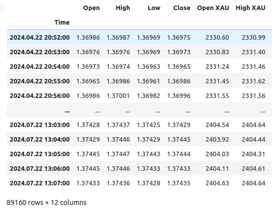
Fig 1: Our merged data frame

Let us define how far into the future we wish to forecast.

#Define the forecast horizon
look_ahead = 20

Define the 3 groups of predictors we wish to test.

#Define the predictors and target
ohlc_predictors = ['Open','High','Low','Close']
new_predictors = ['Open XAU','High XAU','Low XAU','Close XAU','Open XPD','High XPD','Low XPD','Close XPD']
predictors = ohlc_predictors + new_predictors

Labeling the data.

#Let's add labels to the data
merged_data["Target"] = merged_data["Close"].shift(-look_ahead)

Let us also create label’s that will be helpful when we are visualizing the data. These labels will summarize the changes in each market.

#Let's also add labels to help us visualize the relationships
merged_data["Binary Target"] = np.nan
merged_data["XAU Target"] = np.nan
merged_data["XPD Target"] = np.nan

#Define the target values
#Changes in the USDCAD Exchange rate
merged_data.loc[merged_data["Close"] > merged_data["Target"],"Binary Target"] = 0
merged_data.loc[merged_data["Close"] < merged_data["Target"],"Binary Target"] = 1
#Changes in the price of Gold
merged_data.loc[merged_data["Close XAU"] > merged_data["Close XAU"].shift(-look_ahead),"XAU Target"] = 0
merged_data.loc[merged_data["Close XAU"] < merged_data["Close XAU"].shift(-look_ahead),"XAU Target"] = 1
#Changes in the price of Palladium
merged_data.loc[merged_data["Close XPD"] > merged_data["Close XPD"].shift(-look_ahead),"XPD Target"] = 0
merged_data.loc[merged_data["Close XPD"] < merged_data["Close XPD"].shift(-look_ahead),"XPD Target"] = 1

#Drop any NA values
merged_data.dropna(inplace=True)

Exploratory Data Analysis

To visualize our data, we will first import the libraries necessary.

#Explorartory data analysis
import seaborn as sns
import matplotlib.pyplot as plt

Displaying the library versions.

#Display library version
print(f"Seaborn version: {sns.__version__}")

Seaborn version: 0.13.2

First, let us reset the index of our merged data frame.

#Reset the index
merged_data.reset_index(inplace=True)

Now, let us create a correlation heatmap. As we can see, there are significantly strong levels of correlation between the two precious metals and the USDCAD pair. This is inline with our fundamental analysis of the roles played, by these metals, in the Gross Domestic Product of both countries. Unfortunately, this did not result in better performance when attempting to forecast the USDCAD exchange rate.

#Correlation heatmap
fig , ax = plt.subplots(figsize=(7,7))
sns.heatmap(merged_data.loc[:,predictors].corr(),annot=True,ax=ax)

Correlation heatmap

Fig 2: Our correlation heat map

We created two categorical plots summarizing all the instances where the price of Gold or Palladium rose, column 1, or fell, column 2. From there, we colored each of the points to indicate whether the USDCAD exchange rate rose, denoted by the orange dotes, or fell, the blue dots. As one can see, we have a mixture of both outcomes across both columns. Possibly suggesting that the changes in the USDCAD exchange rate are independent of the changes in the precious metals we have picked.

#Let's create categorical plots
sns.catplot(data=merged_data,x="XAU Target",y="Close",hue="Binary Target")

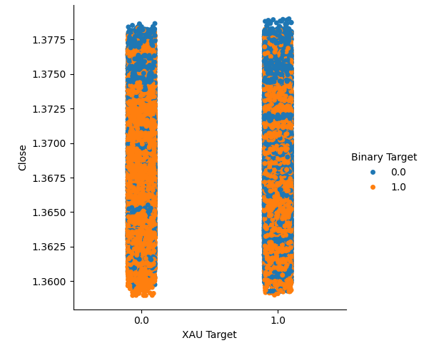
Fig 3: Categorical plot of Gold price and USDCAD close price

#Let's create categorical plots
sns.catplot(data=merged_data,x="XPD Target",y="Close",hue="Binary Target")

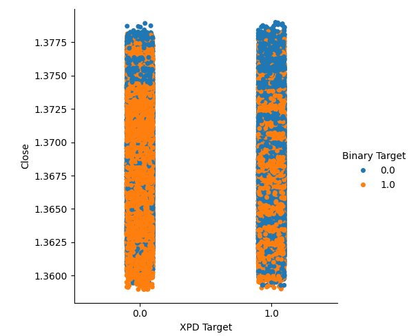
Fig 4: Categorical plot of Palladium price against USDCAD price

Subsequently, we created scatter plots, to visualize the variance between the close price of the Palladium and USDCAD market. Unfortunately, this produced no discernible relationship that we can take advantage of. We colored each point using the same orange and blue color map outlined above.

#Let's visualize scatter plots
sns.scatterplot(data=merged_data,x="Close XPD",y="Close",hue="Binary Target")

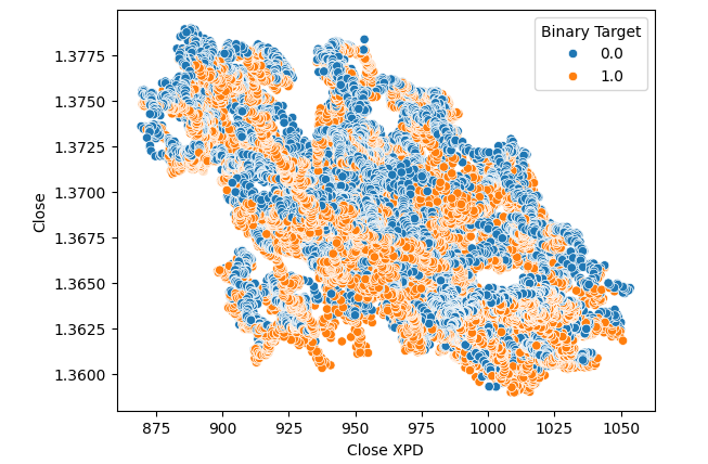
Fig 5: Scatter plot of XPDUSD against USDCAD

No improvements were made when we substituted the price of Gold in place of Palladium in the scatter plot.

#Let's visualize scatter plots
sns.scatterplot(data=merged_data,x="Close XAU",y="Close",hue="Binary Target")

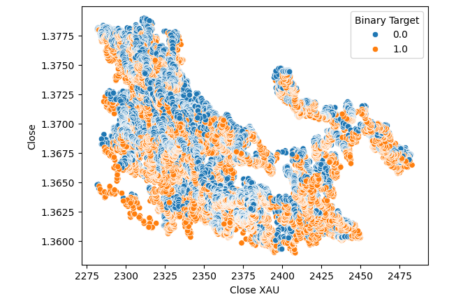
Fig 6: A scatter plot of XAUUSD against USDCAD close

We thought of trying to test for a relationship between the two metals themselves. However, the relationship still was not obvious to us. We created a scatter plot of the price of Gold against the price of Palladium and used the change in the USDCAD pair to color each point, but this made no improvement.

#Let's visualize scatter plots
sns.scatterplot(data=merged_data,x="Close XPD",y="Close XAU",hue="Binary Target")

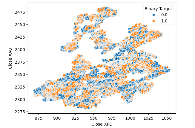
Fig 7: A scatter plot of XAUUSD against XPDUSD

Sometimes, relationships may be hidden since we are not viewing enough variables at the same time to see the effect. We created a 3D scatter plot, using the closing price of Palladium, Gold and the USDCAD. Unfortunately, the resulting plot highlighted what appeared to be clusters in the data that have poor levels of separation, essentially restating what we already know so far.

#Visualizing 3D data
fig = plt.figure(figsize=(7,7))
ax = fig.add_subplot(111,projection='3d')
colors = ['blue' if movement == 0 else 'orange' for movement in merged_data.loc[0:1100,"Binary Target"]]
ax.scatter(merged_data.loc[0:1100,"Close"],merged_data.loc[0:1100,"Close XAU"],merged_data.loc[0:1100,"Close XPD"],c=colors)

#Set labels
ax.set_xlabel('USDCAD')
ax.set_ylabel('XAUUSD')
ax.set_zlabel('XPDUSD')

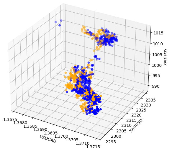
Fig 8: Visualizing our market data in 3D

Data Modeling

Let us get ready to start modelling our data. First, we will import standard libraries.

#Modelling the data
import sklearn
from sklearn.model_selection import train_test_split
from sklearn.preprocessing import RobustScaler

Displaying the library version.

#Print library version
print(f"Sklearn version {sklearn.__version__}")

Sklearn version 1.4.1.post1

Before we start training any models, we need to first scale and standardize the data.

#Scale the data
scaled_data = pd.DataFrame(RobustScaler().fit_transform(merged_data.loc[:,predictors]),columns=predictors)

Now we will split the data into two halves, one for training and optimization and the latter for validation and testing for over fitting.

#Split the data
train_X,test_X,train_y,test_y = train_test_split(scaled_data,merged_data.loc[:,"Target"],shuffle=False,test_size=0.5)

Now import the models.

#Preparing to model the data
from sklearn.model_selection import TimeSeriesSplit
from sklearn.linear_model import LinearRegression
from sklearn.ensemble import RandomForestRegressor , GradientBoostingRegressor , BaggingRegressor
from sklearn.svm import LinearSVR
from sklearn.neighbors import KNeighborsRegressor
from sklearn.neural_network import MLPRegressor
from sklearn.metrics import root_mean_squared_error

Create the time series split object.

#Create the time series split object
tscv = TimeSeriesSplit(gap=look_ahead,n_splits=5)

Store the models in a list so we can iterate over them.

#Create a list of models
models = [
        LinearRegression(),
        RandomForestRegressor(),
        GradientBoostingRegressor(),
        BaggingRegressor(),
        LinearSVR(),
        KNeighborsRegressor(),
        MLPRegressor(hidden_layer_sizes=(100,10))
]

Create a data frame to store our accuracy levels.

#List of models
columns = [
        "Linear Regression",
        "Random Forest",
        "Gradient Boost",
        "Bagging",
        "Linear SVR",
        "K-Neighbors",
        "Neural Network"
]

#Create a dataframe to store our error metrics
ohlc_error = pd.DataFrame(columns=columns,index=np.arange(0,5))
new_error = pd.DataFrame(columns=columns,index=np.arange(0,5))
all_error = pd.DataFrame(columns=columns,index=np.arange(0,5))

Define the predictors to use.

#Setting the current predictors
current_predictors = predictors

Cross-validate each model using the predictors defined above.

#Perform cross validation
for j in np.arange(0,len(models)):
        model = models[j]
        for i,(train,test) in enumerate(tscv.split(train_X)):
        model.fit(train_X.loc[train[0]:train[-1],current_predictors],train_y.loc[train[0]:train[-1]])
        all_error.iloc[i,j] = root_mean_squared_error(train_y.loc[test[0]:test[-1]],model.predict(train_X.loc[test[0]:test[-1],current_predictors]))

Let us observe our error levels using ordinary OHLC data. From our visualizations and the summary statistics, it is clear that the Linear Regression model performed best on this task.

ohlc_error

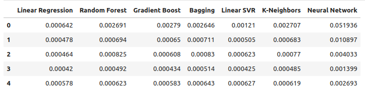
Fig 9: Our error levels when forecasting using OHLC USDCAD data

Plotting the data.

ohlc_error.plot()

Fig 10: Our model accuracy using the first set of predictors

Creating box-plots.

fig = plt.figure(figsize=(5,5))
plt.boxplot(ohlc_error)

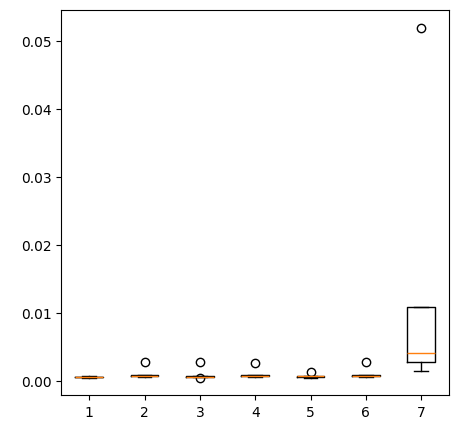
Fig 11: Our model accuracy when forecasting with the first group of predictors

Let us observe our error levels when using the precious metals to forecast the USDCAD exchange rate. The linear regression is still the best performing model, however, no longer by a wide margin.

new_error

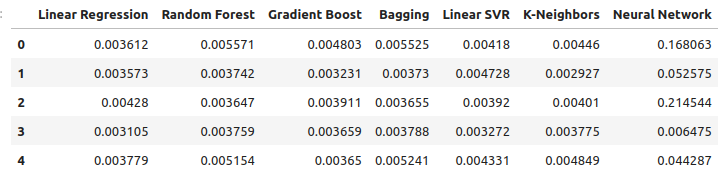
Fig 12: Our new error levels

Plotting the new error levels.

new_error.plot()

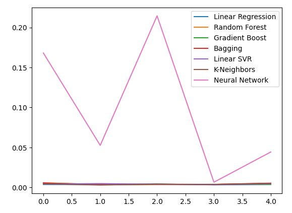
Fig 13: Our new error levels

Creating a box-plot of the new results.

fig = plt.figure(figsize=(5,5))
plt.boxplot(new_error)

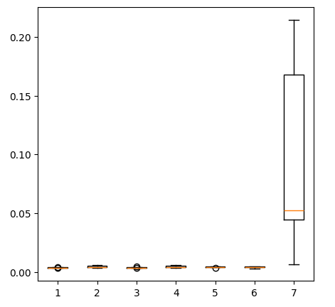
Fig 14: Our error levels when using precious metals market data

Now if let us consider our performance when using all the available data. We still observe that the linear model is performing well ahead of every other model we have. Let us try to optimize the second-best model, the LinearSVR, to outperform the Linear Regression.

all_error

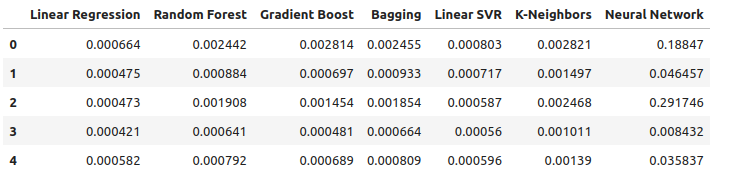
Fig 15: Our accuracy when using all the data we have

Plotting the error levels.

all_error.plot()

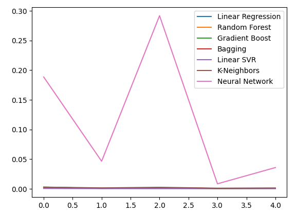
Fig 16: Line plots of our accuracy when using all the data we have

Creating a box-plot of the error levels we obtained when using all the data we have, shows that the simple linear regression is still our best choice.

fig = plt.figure(figsize=(5,5))
plt.boxplot(all_error)

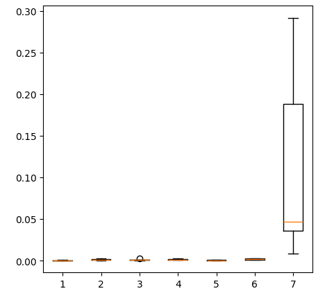
Fig 17: Box-plots of our accuracy when using all the data we have

The mean error levels of our models across all 5 validation sets clearly show the linear model is our best choice so far. However, the LinearSVR is not far behind.

all_error.mean()

Linear Regression 0.000523
Random Forest      0.001333
Gradient Boost       0.001227
Bagging                  0.001343
Linear SVR             0.000653
K-Neighbors            0.001837
Neural Network       0.114188
dtype: object

Feature Importance

Before we start optimizing our model, let us first assess which features appear important, hopefully our data related to the precious metals market will show its value in this test. We will first test the mutual information (MI) levels. MI is a measure of how much certainty you gain about the value of the target, from knowing the value of one of the predictors. MI is on a logarithmic scale, therefore an MI score above 2 is rare to find in practice.

We start by importing the libraries we need.

#Mutual information score
from sklearn.feature_selection import mutual_info_regression

Now we calculate MI scores for each of our predictors.

#Prepare the data for plotting
mi = mutual_info_regression(train_X,train_y)
mi = mi.reshape(1,12)
mi_scores = pd.DataFrame(mi,columns=predictors)

Plotting our MI scores suggests to us that the data from the USDCAD market may be more informative than all the data from the precious metals market. This is validated by our cross validation test, in which we observed the Linear Model using just the Quotes from the USDCAD market produced the lowest error.

#Prepare the data for plotting
mi = mutual_info_regression(train_X,train_y)
mi = mi.reshape(1,12)
mi_scores = pd.DataFrame(mi,columns=predictors)
#Plot the scores
mi_scores.plot.bar()

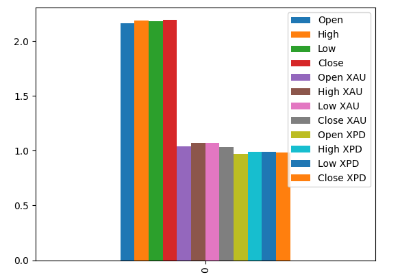
Fig 18: Mutual information scores across our 3 datasets

Next we will calculate SHAP values. SHAP values are black-box explainers that help us identify global feature importance in our machine learning models.

Import the SHAP library.

#The Linear SVR appears to be performing second best
import shap

Initialize the LSVR model.

#Initialize the model
model = LinearSVR()
model.fit(train_X,train_y)

Compute SHAP values.

#Compute SHAP values
explainer = shap.Explainer(model,train_X)
explanations = explainer(train_X)

Show global feature importance.

#Plot SHAP values
shap.plots.violin(explanations)

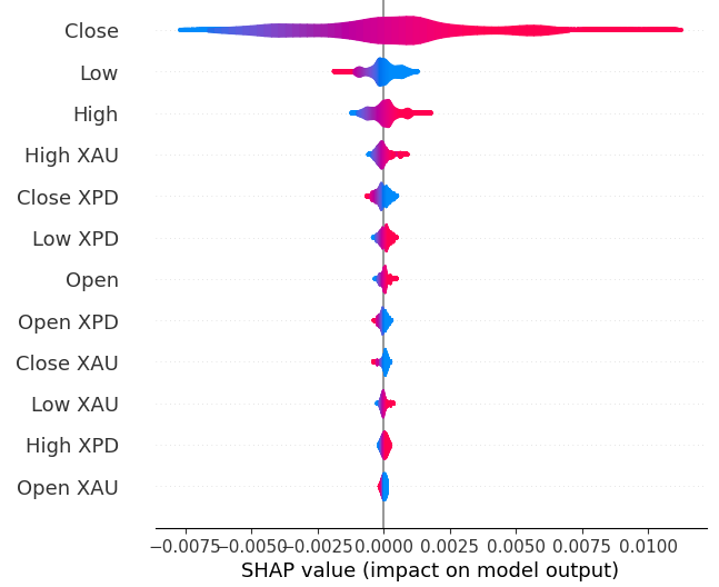
Fig 19: Our SHAP Importance levels

Our SHAP explanations disagree with our Mutual Information assessment. We have covered the disagreement problem extensively in previous articles, the best that can be said is that feature importance can be challenging to assess and must be taken with a grain of salt. However, both explanations suggest there is some useful information contained in the precious metals markets.

Hyperparameter Tuning

Tuning our model may allow us to perform better on unseen data than we would be able to when using the default model.

To tune our model, let us first import the libraries we need.

#Parameter tuning
from sklearn.model_selection import RandomizedSearchCV

Now initialize the model.

#Reinitialize the model
model = LinearSVR()

Then we define our tuning parameters. We pass the model, and a dictionary of possible parameter values, followed by the total number of iterations we wish to perform. We would like to perform 5-fold cross validation to measure the negative mean squared error, this means we will select the model with the lowest validation error. Lastly, setting n_jobs to minus 1 allows performing the search in parallel across all available CPU cores.

#Define the tuner
tuner = RandomizedSearchCV(
        model,
        {
        "epsilon" : [0,10,100,1000],
        "tol":[0.01,0.001,0.0001,0.00001,0.0000001],
        "C":[1,10,100,1000,10000],
        "loss":['epsilon_insensitive', 'squared_epsilon_insensitive']  
        },
        n_iter=1000,
        cv=5,
        n_jobs=-1,
        scoring="neg_mean_squared_error"
)

Fit the tuner.

#Let's fit the tuner
tuner_results = tuner.fit(train_X,train_y)

The best parameters we found.

#Let's see the best parameters we found
tuner_results.best_params_

{'tol': 1e-05, 'loss': 'squared_epsilon_insensitive', 'epsilon': 0, 'C': 10000}

Testing For Over-fitting

To test for over-fitting, we first need to initialize our models.

#Testing for overfitting
benchmark =  LinearRegression()
default_lsvr = LinearSVR()
customized_lsvr = LinearSVR(tol=1e-05,loss='squared_epsilon_insensitive',epsilon=0,C=10000)

Now reset the indexes so we can perform cross validation.

#Reset the indexes
test_y = test_y.reset_index()
test_X = test_X.reset_index()

Format the data.

#Format the data
test_y = test_y.loc[:,"Target"]
test_X = test_X.loc[:,predictors]

Create data frames to store our error levels.

#Create dataframes to store our error levels
test_error = pd.DataFrame(columns=["Linear Regression","LSVR","Customized LSVR"],index=[0,1,2,3,4])

Train the models on the training set.

#Fit the models on the training set
benchmark.fit(train_X,train_y)
default_lsvr.fit(train_X,train_y)
customized_lsvr.fit(train_X,train_y)

Store the models in a list.

models = [benchmark,default_lsvr,customized_lsvr]

Cross-validating each model on the test set.

for j in np.arange(0,len(models)):
        model = models[j]
        for i,(train,test) in enumerate(tscv.split(test_X)):
        model.fit(test_X.loc[train[0]:train[-1],:],test_y.loc[train[0]:train[-1]])
        test_error.iloc[i,j] = root_mean_squared_error(test_y.loc[test[0]:test[-1]],model.predict(test_X.loc[test[0]:test[-1],:]))

Our test error.

test_error

Linear Regression	LSVR	Customized LSVR
0.000598	0.000542	0.000743
0.000472	0.000573	0.000722
0.000318	0.000451	0.000333
0.000341	0.000366	0.000499
0.00043	0.000839	0.00043

According to our average performance across all 5 folds, our linear model was still the best performing model. However, we managed to outperform the default model.

#Let's calculate our mean performances
test_error.mean()

Linear Regression      0.000432
LSVR                  0.000554
Customized LSVR      0.000545
dtype: object

Visualizing our test error.

#Let's visualize our error
test_error.plot()

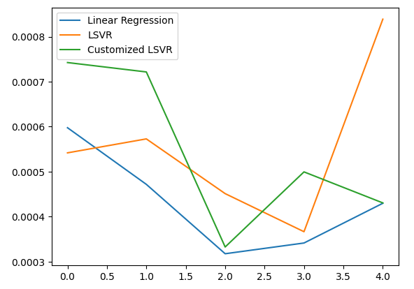
Fig 20: Visualizing our test error

Creating a box plot of our test error rates.

#Create a boxplot of the error
sns.boxplot(data=test_error)

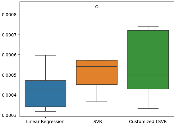
Fig 21: Visualizing our test error

Preparing the Model for Export to ONNX

Before we can export our model to ONNX format, we first need to scale and standardize the data by subtracting the mean and dividing by the standard deviation, from there we will write out our scaling factors to CSV so we can reproduce the procedure in MQL5.

First, create the data frame to store our scaling factors.

#Let's scale our data
scaling_factors = pd.DataFrame(columns=predictors,index=['mean','standard deviation'])
X = merged_data.loc[:,predictors]
y = merged_data.loc[:,"Target"]

Then store the mean and standard deviation, and finally perform the scaling procedure.

#Let's fill each column
for i in np.arange(0,len(predictors)):
        scaling_factors.iloc[0,i] = X.iloc[:,i].mean()
        scaling_factors.iloc[1,i] = X.iloc[:,i].std()
        X.iloc[:,i] = ( ( X.iloc[:,i] - scaling_factors.iloc[0,i] ) / scaling_factors.iloc[1,i])

Save the scaling factors.

#Save the scaling factors as a CSV
scaling_factors.to_csv("/home/volatily/.wine/drive_c/Program Files/MetaTrader 5/MQL5/Files/usd_cad_xau_xpd_scaling_factors.csv")

Exporting the Model to ONNX

ONNX stands for Open Neural Network Exchange (ONNX) and it is an open source, interoperable machine learning framework that allows developers to create, share and deploy machine learning models in a language-agnostic framework. This is accomplished by representing each machine learning model as a tree of nodes and graphs that can be reassembled back to the original model by any language that supports the ONNX API.

First, we shall import the libraries we need.

#Let's prepare to export our model to ONNX format
import onnx
import netron
import skl2onnx
from skl2onnx import convert_sklearn
from skl2onnx.common.data_types import FloatTensorType

Displaying the library versions.

#Display library versions
print(f"Onnx version: {onnx.__version__}")
print(f"Netron version: {netron.__version__}")
print(f"Skl2onnx version: {skl2onnx.__version__}")

Onnx version: 1.15.0
Netron version: 7.8.0
Skl2onnx version: 1.16.0

Now, we shall define our model’s input types.

#Define the input type
initial_types = [('float_input',FloatTensorType([1,12]))]

Let us train the model on all the data we have.

#Train the model on all the data we have
customized_lsvr = LinearSVR(tol=1e-05,loss='squared_epsilon_insensitive',epsilon=0,C=10000)
customized_lsvr.fit(X,y)

Convert the model to ONNX format.

#Covert the sklearn model
onnx_model = convert_sklearn(customized_lsvr,initial_types=initial_types)

Save the ONNX model.

#Save the onnx model
onnx_name = "USDCAD XAUUSD XPDUSD M1 Float.onnx"
onnx.save(onnx_model,onnx_name)

View the ONNX model.

#View the onnx model
netron.start(onnx_name)

Our ONNX model visualized in netron

Fig 22: Visualizing our ONNX model in netron

Our ONNX model parameters in Netron.

Fig 23: Our ONNX model parameters align with our expectations for the model input and output

Implementation in MQL5

For us to implement an AI integrated Expert Advisor in MQL5, we first have to load the ONNX model we exported earlier.

//+------------------------------------------------------------------+
//|                                                    USDCAD AI.mq5 |
//|                                        Gamuchirai Zororo Ndawana |
//|                          https://www.mql5.com/en/gamuchiraindawa |
//+------------------------------------------------------------------+
#property copyright "Gamuchirai Zororo Ndawana"
#property link      "https://www.mql5.com/en/gamuchiraindawa"
#property version   "1.00"

//+------------------------------------------------------------------+
//| Resources                                                        |
//+------------------------------------------------------------------+
#resource  "\\Files\\USDCAD XAUUSD XPDUSD M1 Float.onnx" as const uchar onnx_buffer[];

Next, we must load the trade library so we can open and close positions.

//+------------------------------------------------------------------+
//| Libraries we need                                                |
//+------------------------------------------------------------------+
#include <Trade/Trade.mqh>
CTrade Trade;

Let us also define a few global variables that we will need throughout our program.

//+------------------------------------------------------------------+
//| Global variables                                                 |
//+------------------------------------------------------------------+
long onnx_model;
double mean_values[12],std_values[12];
vectorf model_output = vectorf::Zeros(1);
int model_forecast,state;
double ask,bid;

Let us define helper functions we will use in our program, we need a function responsible for loading our ONNX model and setting its input and output shapes. We will do so using a function that return true if it was successful and false otherwise. Our function first creates the model from the buffer we created earlier, then attempts to set and validate the input and output shapes.

//+------------------------------------------------------------------+
//| This function is responsible for loading our ONNX model          |
//+------------------------------------------------------------------+
bool load_onnx(void)
  {
//--- First we must create the model from the buffer
   onnx_model = OnnxCreateFromBuffer(onnx_buffer,ONNX_DEFAULT);

//--- Now we shall define our I/O shape
   ulong input_shape [] = {1,12};
   ulong output_shape []  = {1,1};

   if(!OnnxSetInputShape(onnx_model,0,input_shape))
        {
        Comment("Failed to set ONNX input shape!");
        return(false);
        }

   if(!OnnxSetOutputShape(onnx_model,0,output_shape))
        {
        Comment("Failed to set ONNX output shape!");
        return(false);
        }

//--- Everything went fine
   return(true);
  }
//+------------------------------------------------------------------+

This function is responsible for reading the CSV file that has our scaling values and storing them into the globally scoped arrays we defined.

//+------------------------------------------------------------------+
//| This function will read our scaling factors and store them       |
//+------------------------------------------------------------------+
bool load_scaling_factors(void)
  {
//--- Read in the file
   string file_name = "usd_cad_xau_xpd_scaling_factors.csv";

//--- Try open the file
   int result = FileOpen(file_name,FILE_READ|FILE_CSV|FILE_ANSI,","); //Strings of ANSI type (one byte symbols).

//--- Check the result
   if(result != INVALID_HANDLE)
        {
        Print("Opened the file");
        //--- Store the values of the file

        int counter = 0;
        string value = "";

        while(!FileIsEnding(result) && !IsStopped()) //read the entire csv file to the end
        {

        if(counter > 100)  //if you aim to read 10 values set a break point after 10 elements have been read
                break; //stop the reading progress

        value = FileReadString(result);
        Print("Trying to read string: ",value," count value: ",counter);

        //--- Check where we are
        if((counter >= 14) && (counter < 26))
        {
                mean_values[counter - 14] = (float) value;
        }
        //--- Check where we are
        if((counter >= 27) && (counter < 39))
        {
                std_values[counter - 27] = (float) value;
        }
        //--- Reading a new row
        if(FileIsLineEnding(result))
        {
                Print("row++");
        }

        counter++;
        }
        //---Close the file
        ArrayPrint(mean_values);
        ArrayPrint(std_values);
        FileClose(result);
        return(true);
        }
//--- We failed to find the file
   else
        {
        Comment("Failed to find the file containing scaling factors");
        return(false);
        }
  }

We also need a function responsible for fetching the updated price quotes from the market.

//+------------------------------------------------------------------+
//| Update market prices                                             |
//+------------------------------------------------------------------+
void update_market_prices(void)
  {
   ask = SymbolInfoDouble(_Symbol,SYMBOL_ASK);
   bid = SymbolInfoDouble(_Symbol,SYMBOL_BID);
  }

Lastly, we need a function for fetching predictions from our model. Our predict function will first scale the data before passing it to our model.

//+------------------------------------------------------------------+
//| Model predict                                                    |
//+------------------------------------------------------------------+
void model_predict(void)
  {
//--- First fetch the market data

   vectorf model_input  =
        {
        iOpen("USDCAD",PERIOD_CURRENT,0),iHigh("USDCAD",PERIOD_CURRENT,0),iLow("USDCAD",PERIOD_CURRENT,0),iClose("USDCAD",PERIOD_CURRENT,0),
        iOpen("XAUUSD",PERIOD_CURRENT,0),iHigh("XAUUSD",PERIOD_CURRENT,0),iLow("XAUUSD",PERIOD_CURRENT,0),iClose("XAUUSD",PERIOD_CURRENT,0),
        iOpen("XPDUSD",PERIOD_CURRENT,0),iHigh("XPDUSD",PERIOD_CURRENT,0),iLow("XPDUSD",PERIOD_CURRENT,0),iClose("XPDUSD",PERIOD_CURRENT,0)
        };

//--- Now standardize and scale the data
   for(int i =0; i < 12; i++)
        {
        model_input[i] = ((model_input[i] - mean_values[i]) / std_values[i]);
        }

//--- Now fetch a prediction from our model
   OnnxRun(onnx_model,ONNX_DEFAULT,model_input,model_output);

//--- Store our model's forecat
   if(model_output[0] > iClose("USDCAD",PERIOD_CURRENT,0))
        {
        model_forecast = 1;
        }
   else
        if(model_output[0] < iClose("USDCAD",PERIOD_CURRENT,0))
        {
        model_forecast = -1;
        }
  }

When initializing our Expert Advisor, we will first load our ONNX file, then read the scaling values. If either one of these procedures fails, we will abort the entire process.

//+------------------------------------------------------------------+
//| Expert initialization function                                   |
//+------------------------------------------------------------------+
int OnInit()
  {
//--- This function will load our ONNX model
   if(!load_onnx())
        {
        return(INIT_FAILED);
        }

//--- This function will load our scaling factors
   if(!load_scaling_factors())
        {
        return(INIT_FAILED);
        }
//---
   return(INIT_SUCCEEDED);
  }

Whenever our Expert Advisor has been removed from the chart, let us free up the resources we no longer need.

//+------------------------------------------------------------------+
//| Expert deinitialization function                                 |
//+------------------------------------------------------------------+
void OnDeinit(const int reason)
  {
//--- Free up the resources we do not need
   OnnxRelease(onnx_model);
   ExpertRemove();
  }

Finally, whenever we receive changes to the bid and ask prices, we will store the updated price in memory and fetch a new prediction from our AI model. If we have no open positions, we will take the position suggested by our AI model, however if we have an open position, we will check to ensure our AI model’s prediction is not going against our current position.

void OnTick()
  {
//--- Update the market prices
   update_market_prices();

//--- Fetch a forecast from our model
   model_predict();

//--- Find a trading oppurtunity
   if(PositionsTotal() == 0)
        {
        if(model_forecast == -1)
        {
        Trade.Sell(0.2,_Symbol,ask,0,0,"USDCAD AI");
        state = -1;
        }

        else
        if(model_forecast == 1)
        {
                Trade.Buy(0.2,_Symbol,ask,0,0,"USDCAD AI");
                state = 1;
        }
        }

//--- Check for reversals
   if(PositionsTotal() > 0)
        {
        if(state != model_forecast)
        {
        Alert("Reversal detected by our AI system, closing all positions now!");
        Trade.PositionClose(_Symbol);
        }
        }

  }
//+------------------------------------------------------------------+

Our system in action

Fig 24: Our expert advisor in action

Our system in action

Fig 25: Our AI system has detected a possible reversal

Conclusion

In today's article, we have demonstrated how you can uncover hidden relationships that may exist between interrelated markets. However, it is worth noting that our empirical analysis shows us that we may be better off using just ordinary market data and simpler linear models. This may be true because, as we all know well, market data can be noisy. And in cases of noisy data, simpler models tend to outperform more complex models because the complex models are sensitive to the variation in the input data.

Attached files |

Download ZIP

RICS_VIII_USDCAD.ipynb (1815.01 KB)

USDCAD_XAUUSD_XPDUSD_M1_Float.onnx (0.32 KB)

USDCAD_AI.mq5 (7.77 KB)

usd_cad_xau_xpd_scaling_factors.csv (0.56 KB)

Warning: All rights to these materials are reserved by MetaQuotes Ltd. Copying or reprinting of these materials in whole or in part is prohibited.