
Neural Networks in Trading: Hierarchical Feature Learning for Point Clouds

Introduction
A geometric set of points represents a collection of points in Euclidean space. As a set, such data must remain invariant to permutations of its elements. Furthermore, the distance metric defines local neighborhoods, which may exhibit varying properties. For instance, point density and other attributes can be heterogeneous across different regions.
In the previous article, we explored the PointNet method, whose core idea is to learn spatial encoding for each point and subsequently aggregate all individual representations into a global signature of the point cloud. However, PointNet does not capture local structure. Yet, using local structure has proven crucial to the success of convolutional architectures. Convolutional models process input data arranged on regular grids and can progressively capture objects at increasingly larger scales along a multi-resolution hierarchy. At lower levels, neurons have smaller receptive fields, whereas at higher levels, they encompass larger regions. The ability to abstract local patterns across this hierarchy enhances generalization.
A similar approach was applied in the PointNet++ model, introduced in the paper "PointNet++: Deep Hierarchical Feature Learning on Point Sets in a Metric Space". The core idea of PointNet++ is to partition the point set into overlapping local regions based on a distance metric in the underlying space. Similar to convolutional networks, PointNet++ extracts local features, capturing fine-grained geometric structures from small regions. These local structures are then grouped into larger elements and processed to derive higher-level representations. This process is repeated iteratively until features for the entire point set are obtained.
When designing PointNet++, the authors addressed two key challenges: partitioning the point set and abstracting point sets or local features through localized feature learning. These challenges are interdependent because partitioning the point set requires maintaining shared structures across segments to enable shared weight learning for local features, similar to convolutional models. The authors selected PointNet as the local learning unit, as it is an efficient architecture for handling unordered point sets and extracting semantic features. Additionally, this architecture is robust to noise in the input data. As a fundamental building block, PointNet abstracts sets of local points or objects into higher-level representations. Within this framework, PointNet++ recursively applies PointNet to nested subdivisions of the input data.
One remaining challenge is the method for creating overlapping partitions of the point cloud. Each region is defined as a neighborhood sphere in Euclidean space, characterized by parameters such as centroid location and scale. To ensure even coverage of the entire set, centroids are selected from the original points using a farthest-point sampling algorithm. Compared to volumetric convolutional models that scan space with fixed strides, the local receptive fields in PointNet++ depend on both the input data and the distance metric. This increases their efficiency.
1. The PointNet++ algorithm
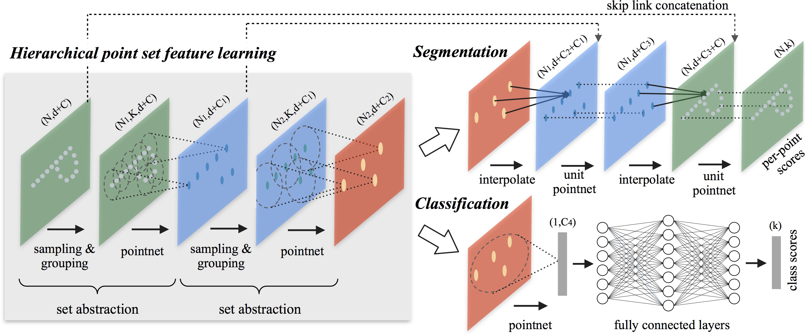
The PointNet architecture uses a single MaxPooling operation to aggregate the entire set of points. In contrast, the authors of PointNet++ introduce a hierarchical architecture that progressively abstracts local regions along multiple levels of hierarchy.
The proposed hierarchical structure consists of several predefined abstraction levels. At each level, the point cloud is processed and abstracted to create a new dataset with fewer elements. Each abstraction level comprises three key layers: Sampling Layer, Grouping Layer, and PointNet Layer. The Sampling Layer selects a subset of points from the original point cloud, defining the centroids of local regions. The Grouping Layer then forms local point sets by identifying "neighboring" points around each centroid. Finally, the PointNet Layer applies a mini-PointNet to encode local patterns into feature vectors.
The abstraction level takes an input matrix of size N×(d+C), where N is the number of points, d is the dimensionality of coordinates and C is the dimensionality of features. It outputs a matrix of size N′×(d+C′), where N′ is the number of subsampled points, and C′ is the dimensionality of the new feature vector that encapsulates the local context.
The authors of PointNet++ propose iterative farthest point sampling (FPS) to select a subset of centroid points. Compared to random sampling, this method provides better coverage of the entire point cloud while maintaining the same number of centroids. Unlike convolutional networks, which scan vector space independently of data distribution, this sampling strategy generates receptive fields that are inherently data-dependent.
The Grouping Layer takes as input a point cloud of size N×(d+C) and a set of centroid coordinates of size N′×d. The output consists of grouped point sets of size N′×K×(d+C), where each group corresponds to a local region and K is the number of points within the centroid's neighborhood.
Note that K varies from group to group, but the subsequent PointNet Layer can transform a flexible number of points into a fixed-length feature vector representing the local region.
In convolutional neural networks (CNNs), a pixel’s local neighborhood consists of adjacent pixels within a defined Manhattan distance (kernel size). In a point cloud, where points exist in metric space, neighborhood relations are determined by the distance metric.
During the grouping process, the model identifies all points that lie within a predefined radius of the query point (with K capped as a hyperparameter).
In the PointNet Layer, the input consists of N′ local regions with a data size of N′×K×(d+C). Each local region is ultimately abstracted into its centroid and a corresponding local feature that encodes its surrounding neighborhood. The resulting tensor size is N′×(d+C).
The coordinates of points within each local region are first transformed into a local coordinate system relative to their centroid:
![]()
for i = 1, 2,…, K ad j = 1, 2,…, d, where ![]() represents the centroid's coordinates.
represents the centroid's coordinates.
The authors of PointNet++ use PointNet as the fundamental building block for learning local patterns. By using relative coordinates along with individual point features, the model effectively captures relationships between points within a local region.
Often point clouds have non-uniform point density across different regions. This heterogeneity poses a significant issue when learning point set features. Features learned in densely sampled areas may not generalize well to sparsely populated region. Consequently, models trained on sparse point clouds may fail to recognize fine-grained local structures.
Ideally, point cloud processing should be as precise as possible to capture the finest details in densely sampled regions. However, such detailed analysis is inefficient in areas with low point density, as local patterns can be distorted due to insufficient data. In these cases, a broader neighborhood must be considered to detect larger-scale structures. To address this, the authors of PointNet++ propose density-adaptive PointNet layers, which are designed to aggregate features from multiple scales while accounting for variations in point density.
Each abstraction level in PointNet++ extracts multiple scales of local patterns and intelligently combines them based on local point density. The original paper presents two types of density-adaptive layers.
A straightforward yet effective approach to capturing multi-scale patterns involves applying multiple grouping layers with different scales and assigning corresponding PointNet modules to extract features at each scale. The resulting multi-scale representations are then combined into a unified feature.
The network learns an optimal strategy for merging multi-scale features. This is achieved by randomly dropping input points with a probability assigned to each instance.
The approach described above demands significant computational resources, as it applies local PointNet operations within large-scale neighborhoods for each centroid point. To mitigate this computational overhead while preserving the ability to adaptively aggregate information, the authors propose an alternative feature fusion method based on concatenating two feature vectors. One vector is derived by aggregating features from each subregion at the lower level Li-1 using the given abstraction level. The second vector is obtained by directly processing all original points within a local region using a single PointNet module.
When the local region density is low, the first vector may be less reliable than the second, as the subregion used for feature computation contains even fewer points and is more affected by sparse sampling. In this case, the second vector should have a higher weight. Conversely, when point density is high, the first vector provides more fine-grained details, as it can recursively examine local structures with higher resolution at lower levels.
This method is computationally more efficient, as it avoids computing features for large-scale neighborhoods at the lowest levels.
In the abstraction layer, the original point set undergoes subsampling. However, in segmentation tasks such as semantic point labeling, it is desirable to obtain per-point features for all original points. One possible solution is to sample all points as centroids across all abstraction levels, but this significantly increases computational costs. Another way is to propagate objects from the subsampled points to the original ones.
Author's visualization of the PointNet++ method is presented below.
2. Implementation in MQL5
After reviewing the theoretical aspects of the PointNet++ method, we now move on to the practical part of our article, where we implement our interpretation of the proposed approaches using MQL5. It is worth noting that our implementation differs in some respects from the original version described above. But first things first.
We'll divide our work into two main sections. First, we will create a local subsampling layer, which will integrate the Sampling and Grouping layers discussed earlier. Then, we will develop a high-level class that will assemble the individual components into a complete PointNet++ algorithm.
2.1 Extending the OpenCL program
The local subsampling algorithm will be implemented in the CNeuronPointNet2Local class. However, before we begin working on this class, we must first extend the functionality of our OpenCL program.
To start, we will create the CalcDistance kernel, which will compute the distances between points in the analyzed point cloud.
It is important to note that distances will be calculated in a multidimensional feature space, where each point is represented by a feature vector. The kernel’s output will be an N×N matrix with zero values along the diagonal.
The kernel parameters will include pointers to two data buffers (one for the input data and one for storing the results) and a constant that specifies the dimensionality of the point feature vector.
__kernel void CalcDistance(__global const float *data,
                           __global float *distance,
                           const int dimension
                          )
  {
   const size_t main = get_global_id(0);
   const size_t slave = get_local_id(1);
   const int total = (int)get_local_size(1);
Inside the kernel, we identify the thread within the task space.
Our expected output is a square matrix. Therefore, we define a two-dimensional task space of the appropriate size. This ensures that each individual thread computes a single element of the resulting matrix.
At this point, we introduce the first deviation from the original PointNet++ algorithm. We will not iteratively determine centroids for local regions. Instead, our implementation treats each point in the cloud as a centroid. To implement adaptability in region sizes, we normalize the distances to each point in the cloud. Normalizing distances requires data exchange between individual threads. To facilitate this, we organize local workgroups along the rows of the result matrix.
For efficient data exchange within a workgroup, we create a local array.
   __local float Temp[LOCAL_ARRAY_SIZE];
   int ls = min((int)total, (int)LOCAL_ARRAY_SIZE);
Then we determine the offset constants to the required elements in the data buffers.
   const int shift_main = main * dimension;
   const int shift_slave = slave * dimension;
   const int shift_dist = main * total + slave;
After that, we create a loop for calculating the distance between two objects in a multidimensional space.
//--- calc distance
   float dist = 0;
   if(main != slave)
     {
      for(int d = 0; d < dimension; d++)
         dist += pow(data[shift_main + d] - data[shift_slave + d], 2.0f);
     }
Please note that the calculations are performed only for off-diagonal elements. This is because the distance from a point to itself is equal to "0". So, we don't waste resources on unnecessary calculations.
The next step is to determine the maximum distance within the working group. First, we collect the maximum values of individual blocks into a local array.
//--- Look Max
   for(int i = 0; i < total; i += ls)
     {
      if(!isinf(dist) && !isnan(dist))
        {
         if(i <= slave && (i + ls) > slave)
            Temp[slave - i] = max((i == 0 ? 0 : Temp[slave - i]), dist);
        }
      else
         if(i == 0)
            Temp[slave] = 0;
      barrier(CLK_LOCAL_MEM_FENCE);
     }
Then we find the maximum value in the array.
   int count = ls;
   do
     {
      count = (count + 1) / 2;
      if(slave < count && (slave + count) < ls)
        {
         if(Temp[slave] < Temp[slave + count])
            Temp[slave] = Temp[slave + count];
         Temp[slave + count] = 0;
        }
      barrier(CLK_LOCAL_MEM_FENCE);
     }
   while(count > 1);
After finding the maximum value to the analyzed point, we divide the distances calculated above by it. As a result, all distances between points will be normalized in the range [0, 1].
//--- Normalize
   if(Temp[0] > 0)
      dist /= Temp[0];
   if(isinf(dist) || isnan(dist))
      dist = 1;
//--- result
   distance[shift_dist] = dist;
  }
We save the computed value in the corresponding element of the global result buffer.
Of course, we recognize that the maximum distance between two points in the analysis will likely vary. By normalizing values within different scales, we lose this difference. However, this is precisely what enables the adaptation of receptive fields.
If the analyzed point is located within a dense region of the cloud, the farthest point from it is typically situated at one of the cloud's boundaries. Conversely, if the analyzed point is on the edge of the cloud, the farthest point lies at the opposite boundary. In the second case, the distance between the points will be greater. Consequently, the receptive field in the second case will be larger.
We also assume that point density is higher within the cloud than at its edges. Given this, increasing receptive fields at the cloud's periphery is a justified approach to ensure meaningful feature extraction.
The authors of PointNet++ propose computing local point displacements relative to their centroids and then applying mini-PointNet to these local subsets. However, despite its apparent simplicity, this method presents a significant implementation problem.
As previously mentioned, the number of elements in each local region varies and is unknown in advance. This raises an issue regarding buffer allocation. A possible solution is to set a maximum number of points per receptive field and allocate a buffer with excess capacity. However, this would lead to higher memory consumption and increased computational complexity. As a result, training becomes more difficult and model performance is reduced.
Instead, we adopted a simpler and more universal approach. We eliminated the computation of local displacements. To train point features, we use a single weight matrix to all elements, similar to the vanilla PointNet. However, MaxPooling can be implemented within receptive fields. To achieve this, we create a new kernel FeedForwardLocalMax, which takes three buffer pointers as parameters: point feature matrix, normalized distance matrix, and result buffer. Additionally, we introduce a constant for the receptive field radius.
__kernel void FeedForwardLocalMax(__global const float *matrix_i,
                                  __global const float *distance,
                                  __global float *matrix_o,
                                  const float radius
                                 )
  {
   const size_t i = get_global_id(0);
   const size_t total = get_global_size(0);
   const size_t d = get_global_id(1);
   const size_t dimension = get_global_size(1);
We plan the execution of the kernel in a two-dimensional task space. In the first dimension, we indicate the number of elements in the point cloud, and in the second, the dimension of the features of one element. In the kernel body, we immediately identify the current thread in both dimensions of the task space. In this case, each thread works independently, and thus we do not need to create work groups and exchange data between threads.
Next, we define offset constants in data buffers.
   const int shift_dist = i * total;
   const int shift_out = i * dimension + d;
Then we create a loop to determine the maximum value.
   float result = -3.402823466e+38;
   for(int k = 0; k < total; k++)
     {
      if(distance[shift_dist + k] > radius)
         continue;
      int shift = k * dimension + d;
      result = max(result, matrix_i[shift]);
     }
   matrix_o[shift_out] = result;
  }
Pay attention that before checking the value of the next element, we first verify whether it falls within the receptive field of the corresponding point in the cloud.
Once the loop iterations are complete, we store the computed value in the result buffer.
Similarly, we implement the backpropagation kernel CalcInputGradientLocalMax, which distributes the error gradient to the corresponding elements. The feed-forward and backpropagation pass kernels share many similarities. I encourage you to review them independently. You can find the full kernel code in the attachment. Now, we proceed to the main program implementation.
2.2 Local Subsampling Class
Having completed the preparatory work on the OpenCL side, we now turn to developing the local subsampling class. While implementing the OpenCL kernels, we have already touched upon the fundamental principles of algorithm design. However, as we proceed with the CNeuronPointNet2Local class implementation, we will explore these principles in greater detail and examine their practical implementation in code. The structure of the new class is shown below.
class CNeuronPointNet2Local   :  public CNeuronConvOCL
  {
protected:
   float                fRadius;
   uint                 iUnits;
   //---
   CBufferFloat         cDistance;
   CNeuronConvOCL       cFeatureNet[3];
   CNeuronBatchNormOCL  cFeatureNetNorm[3];
   CNeuronBaseOCL       cLocalMaxPool;
   CNeuronConvOCL       cFinalMLP;
   //---
   virtual bool         CalcDistance(CNeuronBaseOCL *NeuronOCL);
   virtual bool         LocalMaxPool(void);
   virtual bool         LocalMaxPoolGrad(void);
   //---
   virtual bool      feedForward(CNeuronBaseOCL *NeuronOCL) override ;
   //---
   virtual bool      calcInputGradients(CNeuronBaseOCL *NeuronOCL) override;
   virtual bool      updateInputWeights(CNeuronBaseOCL *NeuronOCL) override;

public:
                     CNeuronPointNet2Local(void) {};
                    ~CNeuronPointNet2Local(void) {};
   //---
   virtual bool      Init(uint numOutputs, uint myIndex, COpenCLMy *open_cl,
                          uint window, uint units_count, uint window_out, float radius,
                          ENUM_OPTIMIZATION optimization_type, uint batch);
   //---
   virtual int       Type(void) override   const   {  return defNeuronPointNet2LocalOCL; }
   //---
   virtual bool      Save(int const file_handle) override;
   virtual bool      Load(int const file_handle) override;
   //---
   virtual bool      WeightsUpdate(CNeuronBaseOCL *source, float tau) override;
   virtual void      SetOpenCL(COpenCLMy *obj) override;
  };
In the structure presented above, we can observe several internal neural layer objects and two variables, the purpose of which we will explore during the implementation of the class methods.
We also see a familiar set of overridable methods. Additionally, there are three methods that correspond to the previously implemented kernels:
- CalcDistance(CNeuronBaseOCL *NeuronOCL);
- LocalMaxPool(void);
- LocalMaxPoolGrad(void).
As you may have guessed, these methods enqueue the execution of the kernels. Since we have already examined this algorithm in detail, we will not delve into it further in this article.
It is also worth noting that this class inherits from the convolutional layer class CNeuronConvOCL. This is an uncommon practice in our work and is primarily due to the independent processing of features in local groups.
All internal objects of the class are declared statically, which allows us to leave the class constructor and destructor empty. The initialization of a new object instance is handled within the Init method.
bool CNeuronPointNet2Local::Init(uint numOutputs, uint myIndex, COpenCLMy *open_cl,
                                 uint window, uint units_count, uint window_out, float radius,
                                 ENUM_OPTIMIZATION optimization_type, uint batch)
  {
   if(!CNeuronConvOCL::Init(numOutputs, myIndex, open_cl, 128, 128, window_out,
                                        units_count, 1, optimization_type, batch))
      return false;
In the method parameters, we receive the key constants that define the architecture of the object. These parameters closely resemble those used in a convolutional layer. There is one additional parameter: radius, which defines the receptive field radius of an element.
Within the method body, we immediately call the corresponding method of the parent class, where the necessary data validation and initialization of inherited objects have already been implemented. It is important to note that the values passed to the parent class method differ slightly from those received from the external program. This discrepancy arises due to the specific usage of parent class objects, a topic we will revisit when implementing the feedForward method.
After successfully executing the parent class method, we store some of the received constants, while others have already been saved during the parent class operations.
   fRadius = MathMax(0.1f, radius);
   iUnits = units_count;
Next, we move on to initializing the internal objects. First, we create a buffer for recording distances between objects in the analyzed point cloud. As mentioned above, it is a square matrix.
   cDistance.BufferFree();
   if(!cDistance.BufferInit(iUnits * iUnits, 0) ||
      !cDistance.BufferCreate(OpenCL))
      return false;
To extract point features, we create a block of 3 convolutional layers and 3 batch normalization layers, similar to the feature extraction block of the PointNet algorithm. We do not create a source data projection block, since we assume that it is present in the top-level class.
   if(!cFeatureNet[0].Init(0, 0, OpenCL, window, window, 64, iUnits, 1, optimization, iBatch))
      return false;
   if(!cFeatureNetNorm[0].Init(0, 1, OpenCL, 64 * iUnits, iBatch, optimization))
      return false;
   cFeatureNetNorm[0].SetActivationFunction(LReLU);
   if(!cFeatureNet[1].Init(0, 2, OpenCL, 64, 64, 128, iUnits, 1, optimization, iBatch))
      return false;
   if(!cFeatureNetNorm[1].Init(0, 3, OpenCL, 128 * iUnits, iBatch, optimization))
      return false;
   cFeatureNetNorm[1].SetActivationFunction(LReLU);
   if(!cFeatureNet[2].Init(0, 4, OpenCL, 128, 128, 256, iUnits, 1, optimization, iBatch))
      return false;
   if(!cFeatureNetNorm[2].Init(0, 5, OpenCL, 256 * iUnits, iBatch, optimization))
      cFeatureNetNorm[2].SetActivationFunction(None);
Next, we create a layer for recording local MaxPooling results.
   if(!cLocalMaxPool.Init(0, 6, OpenCL, cFeatureNetNorm[2].Neurons(), optimization, iBatch))
      return false;
We add one layer of the resulting MLP.
   if(!cFinalMLP.Init(0, 7, OpenCL, 256, 256, 128, iUnits, 1, optimization, iBatch))
      return false;
   cFinalMLP.SetActivationFunction(LReLU);
We plan to use inherited functionality as the second layer.
Please note that, unlike vanilla PointNet, we use convolutional layers at the output. This is due to the independent processing of local area descriptors.
At the end of the initialization method operations, we explicitly indicate that there is no activation function for our class and return the boolean result of the operations to the calling program.
   SetActivationFunction(None);
   return true;
  }
After completing the work on initializing the new object, we move on to constructing feed-forward pass algorithms in the feedForward method. In the parameters of this method, we receive a pointer to the source data object.
bool CNeuronPointNet2Local::feedForward(CNeuronBaseOCL *NeuronOCL)
  {
   if(!CalcDistance(NeuronOCL))
      return false;
As mentioned above, within this class, we do not plan to project data into a canonical space. It is assumed that this operation will be performed at the top level if necessary. Therefore, we immediately calculate the distance between the elements of the original data.
Next, we create a loop to calculate the features of the analyzed elements.
   CNeuronBaseOCL *temp = NeuronOCL;
   uint total = cFeatureNet.Size();
   for(uint i = 0; i < total; i++)
     {
      if(!cFeatureNet[i].FeedForward(temp))
         return false;
      if(!cFeatureNetNorm[i].FeedForward(cFeatureNet[i].AsObject()))
         return false;
      temp = cFeatureNetNorm[i].AsObject();
     }
Run MaxPooling operations for local areas of points.
   if(!LocalMaxPool())
      return false;
At the end of the method operations, we apply an independent two-layer MLP to the descriptors of all local regions.
   if(!cFinalMLP.FeedForward(cLocalMaxPool.AsObject()))
      return false;
   if(!CNeuronConvOCL::feedForward(cFinalMLP.AsObject()))
      return false;
//---
   return true;
  }
As the first layer of the MLP, we use the internal layer cFinalMLP. The operations of the second layer are performed using the functionality inherited from the parent class.
Do not forget to monitor the operations processes at every stage. After successfully completing all operations, we return a logical result to the calling program.
The backpropagation algorithms are implemented in the methods calcInputGradients and updateInputWeights. The calcInputGradients method distributes the error gradient to all elements according to their impact on the final result. The algorithm follows the same logic as the feedForward method but executes the operations in reverse order. The updateInputWeights method updates the trainable parameters of the model. Here, we simply call the corresponding methods of the internal objects that contain the trainable parameters. Both methods are quite simple. I encourage you to explore their implementations independently. The full source code for this class and all its methods can be found in the attachment.
2.3 Assembling the PointNet++ Algorithm
We've completed most of the work. Now we're approaching the final stage of our implementation. At this step, we will combine the individual components into a unified PointNet++ algorithm. This integration will take place within the CNeuronPointNet2OCL class, whose structure is outlined below.
class CNeuronPointNet2OCL   :  public CNeuronPointNetOCL
  {
protected:
   CNeuronPointNetOCL   *cTNetG;
   CNeuronBaseOCL       *cTurnedG;
   //---
   CNeuronPointNet2Local caLocalPointNet[2];
   //---
   virtual bool      feedForward(CNeuronBaseOCL *NeuronOCL) override ;
   //---
   virtual bool      calcInputGradients(CNeuronBaseOCL *NeuronOCL) override;
   virtual bool      updateInputWeights(CNeuronBaseOCL *NeuronOCL) override;
public:
                     CNeuronPointNet2OCL(void) {};
                    ~CNeuronPointNet2OCL(void) ;
   //---
   virtual bool      Init(uint numOutputs, uint myIndex, COpenCLMy *open_cl,
                          uint window, uint units_count, uint output, bool use_tnets,
                          ENUM_OPTIMIZATION optimization_type, uint batch);
   //---
   virtual int       Type(void) override   const   {  return defNeuronPointNet2OCL; }
   //---
   virtual bool      Save(int const file_handle) override;
   virtual bool      Load(int const file_handle) override;
   //---
   virtual bool      WeightsUpdate(CNeuronBaseOCL *source, float tau) override;
   virtual void      SetOpenCL(COpenCLMy *obj) override;
  };
Strangely enough, this class declares only two static objects for local data discretization and two dynamic objects, which are initialized only if data projection into canonical space is required. This simplicity is achieved by inheriting from the vanilla PointNet class, where most of the functionality has already been implemented.
As mentioned earlier, dynamic objects are initialized only when needed. Therefore, we keep the constructor empty, but in the destructor, we check for valid pointers to dynamic objects and delete them if necessary.
CNeuronPointNet2OCL::~CNeuronPointNet2OCL(void)
  {
   if(!!cTNetG)
      delete cTNetG;
   if(!!cTurnedG)
      delete cTurnedG;
  }
Initialization of the class object, as usual, is implemented in the Init method. In the method parameters, we receive the key constants that define the class architectures. We have completely preserved them from the parent class.
bool CNeuronPointNet2OCL::Init(uint numOutputs, uint myIndex, COpenCLMy *open_cl,

                               uint window, uint units_count, uint output, bool use_tnets,
                               ENUM_OPTIMIZATION optimization_type, uint batch)
  {
   if(!CNeuronPointNetOCL::Init(numOutputs, myIndex, open_cl, 64, units_count,
                                output, use_tnets, optimization_type, batch))
      return false;
In the method body, we immediately call a similar method of the parent class. After that, we check whether we need to create projection objects of the original data into the canonical space.
//--- Init T-Nets
   if(use_tnets)
     {
      if(!cTNetG)
        {
         cTNetG = new CNeuronPointNetOCL();
         if(!cTNetG)
            return false;
        }
      if(!cTNetG.Init(0, 0, OpenCL, window, units_count, window * window, false, optimization, iBatch))
         return false;
If necessary, we first create the necessary objects and then initialize them.
      if(!cTurnedG)
        {
         cTurnedG = new CNeuronBaseOCL();
         if(!cTurned1)
            return false;
        }
      if(!cTurnedG.Init(0, 1, OpenCL, window * units_count, optimization, iBatch))
         return false;
     }
If the user has not indicated the need to create projection objects, then we check if there are current pointers to the objects. If there are such pointers, we remove unnecessary objects.
   else
     {
      if(!!cTNetG)
         delete cTNetG;
      if(!!cTurnedG)
         delete cTurnedG;
     }
We then initialize 2 local data sampling objects with different receptive window radii. Complete the method execution.
   if(!caLocalPointNet[0].Init(0, 0, OpenCL, window, units_count, 64, 0.2f, optimization, iBatch))
      return false;
   if(!caLocalPointNet[1].Init(0, 0, OpenCL, 64, units_count, 64, 0.4f, optimization, iBatch))
      return false;
//---
   return true;
  }
Note that we start with a small receptive window and then increase it. However, we do not increase the receptive window to full coverage, since this is performed by the functionality inherited from the vanilla PointNet class.
After completing the work with the class object initialization method, we move on to constructing the feed-forward pass algorithm within the feedForward method.
bool CNeuronPointNet2OCL::feedForward(CNeuronBaseOCL *NeuronOCL)
  {
//--- LocalNet
   if(!cTNetG)
     {
      if(!caLocalPointNet[0].FeedForward(NeuronOCL))
         return false;
     }
In the method parameters, we receive a pointer to the source data object. In the method body, we first check whether projection into canonical space is required. The procedure here is similar to the approach used in the vanilla PointNet class. If data projection is not required, we immediately pass the received pointer to the feedForward method of the first local discretization layer.
Otherwise, we first generate the projection matrix for the data.
   else
     {
      if(!cTurnedG)
         return false;
      if(!cTNetG.FeedForward(NeuronOCL))
         return false;
After that, we implement the projection of the original data by multiplying it by the projection matrix.
      int window = (int)MathSqrt(cTNetG.Neurons());
      if(IsStopped() ||
         !MatMul(NeuronOCL.getOutput(), cTNetG.getOutput(), cTurnedG.getOutput(),
                                    NeuronOCL.Neurons() / window, window, window))
         return false;
Only then do we pass the obtained values to the feed-forward method of the data discretization layer.
      if(!caLocalPointNet[0].FeedForward(cTurnedG.AsObject()))
         return false;
     }
Next, we perform discretization with a larger receptive window size.
   if(!caLocalPointNet[1].FeedForward(caLocalPointNet[0].AsObject()))
      return false;
At the last stage, we pass the enriched data to the feed-forward method of the parent class, where the descriptor of the analyzed point cloud as a whole is determined.
   if(!CNeuronPointNetOCL::feedForward(caLocalPointNet[1].AsObject()))
      return false;
//---
   return true;
  }
As you can see, thanks to the complex inheritance structure, we have managed to construct a concise feedForward method for our new class. The backpropagation methods follow similarly implementations, which I encourage you to explore independently in the attached files. The full code for all programs used in this article is included in the attachment. This includes complete training scripts for the models and their interaction with the environment. It is worth noting that these scripts have been carried over unchanged from the previous article. Moreover, we have largely preserved the model architecture. In fact, the only modification in the environment state encoder was changing the type of a single layer while keeping all other parameters intact.
//--- layer 2
   if(!(descr = new CLayerDescription()))
      return false;
   descr.type = defNeuronPointNet2OCL;
   descr.window = BarDescr;                        // Variables
   descr.count = HistoryBars;                      // Units
   descr.window_out = LatentCount;                 // Output Dimension
   descr.step = int(true);                         // Use input and feature transformation
   descr.batch = 1e4;
   descr.activation = None;
   descr.optimization = ADAM;
   if(!encoder.Add(descr))
     {
      delete descr;
      return false;
     }
This makes it even more interesting to evaluate the Actor's new policy training results.
3. Testing
With this, we have completed our implementation of the approaches proposed by the authors of PointNet++. Now, it is time to evaluate the effectiveness of our implementation using real historical data. As before, we will train the models on historical EURUSD data for the entire year 2023. We use an H1 timeframe. All indicator parameters are set to their default values. The trained model is tested using the MetaTrader 5 strategy tester.
As mentioned earlier, our new model differs from the previous one by only a single layer. Furthermore, this new layer is merely an improved version of our prior work. This makes it particularly interesting to compare the performance of both models. To ensure a fair comparison, we will train both models on the exact same dataset used in the previous experiment.
I always emphasize that updating the training dataset periodically is crucial for achieving optimal model performance. Keeping the dataset aligned with the Actor's current policy ensures a more accurate evaluation of its actions, leading to policy refinements. However, in this case, I couldn’t resist the opportunity to compare two similar approaches and assess the effectiveness of a hierarchical method. In our previous article, we successfully trained an actor policy that was capable of generating profit. We expect the new model to perform at least as well.
After training, our new model successfully learned a profitable policy, achieving positive returns on both training and test datasets. The test results for the new model are presented below.
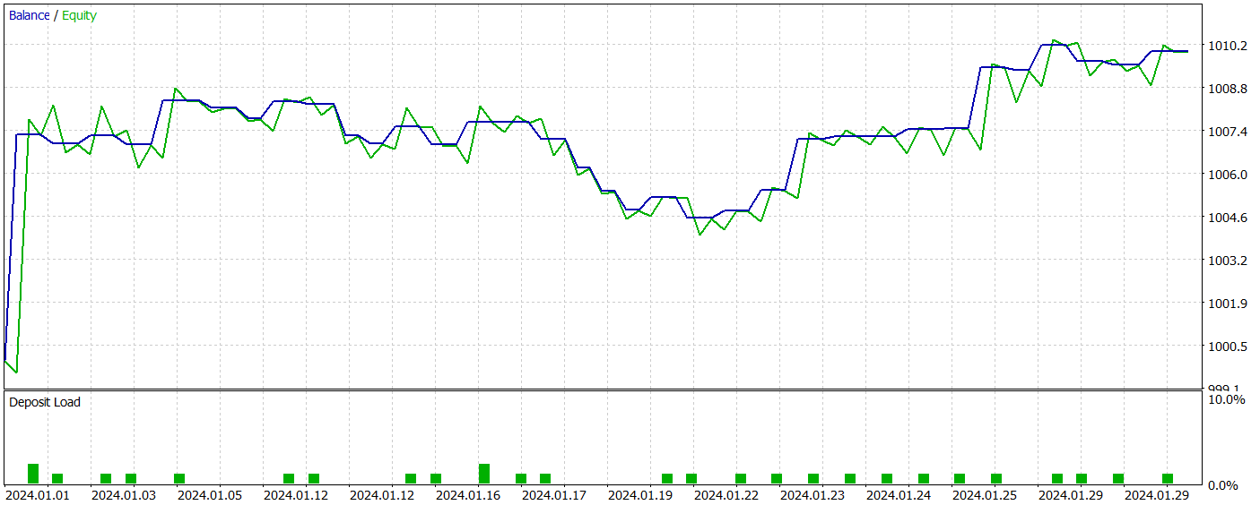
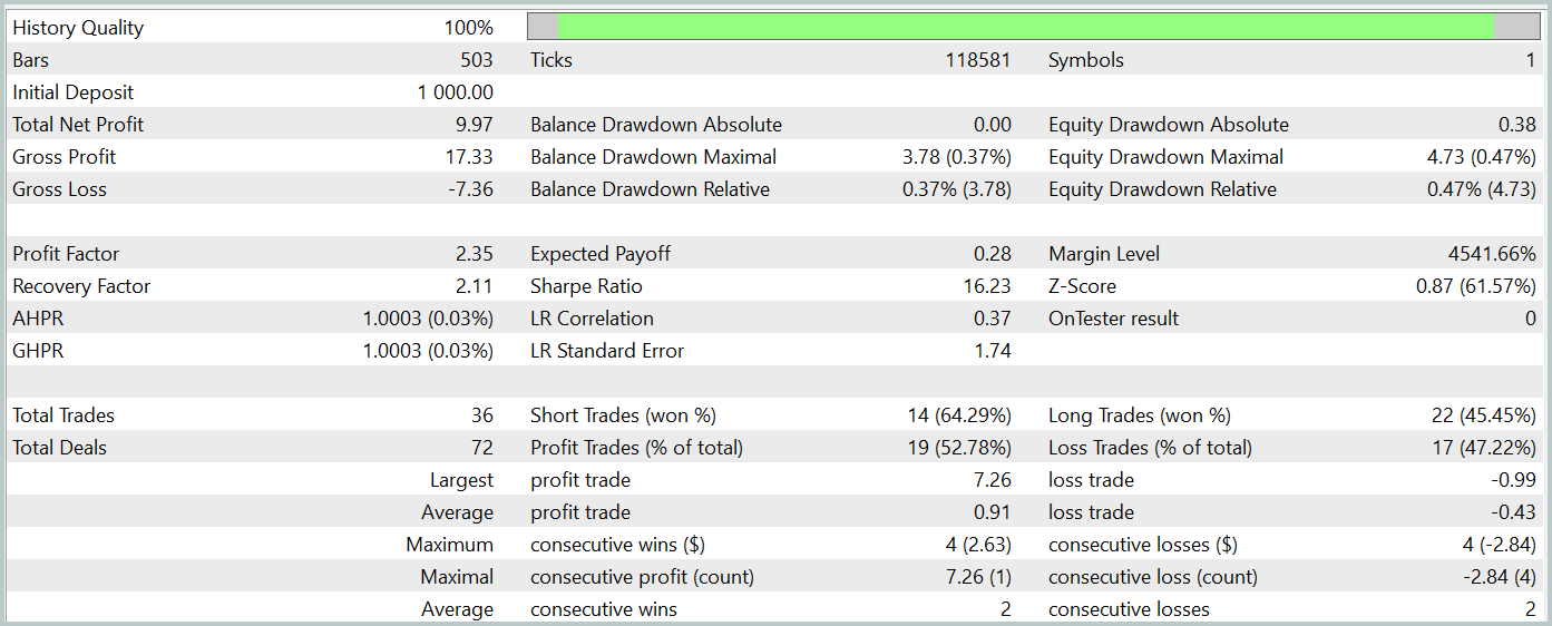
I must admit that comparing the results of both models is quite challenging. Over the test period, both models generated nearly the same profit. Drawdown deviations in both balance and equity remain within a negligible margin of error. However, the new model executed fewer trades, leading to a slight increase in the profit factor.
That being said, the low number of trades executed by both models does not allow us to draw definitive conclusions about their long-term performance.
Conclusion
The PointNet++ method provides an efficient way to analyze both local and global patterns in complex financial data, while accounting for their multidimensional structure. The enhanced approach to point cloud processing improves forecasting accuracy and stability in trading strategies, potentially leading to more informed and successful decision-making in dynamic markets.
In the practical section of this article, we implemented our own vision of the PointNet++ approach. During testing, the model demonstrated its ability to generate profit on the test dataset. However, it is important to note that the presented programs are for demonstration purposes only and are intended solely to illustrate the method operations.
References
- PointNet++: Deep Hierarchical Feature Learning on Point Sets in a Metric Space
- Other articles from this series
| # | Issued to | Type | Description |
|---|---|---|---|
| 1 | Research.mq5 | Expert Advisor | EA for collecting examples |
| 2 | ResearchRealORL.mq5 | Expert Advisor | EA for collecting examples using the Real-ORL method |
| 3 | Study.mq5 | Expert Advisor | Model training EA |
| 4 | Test.mq5 | Expert Advisor | Model testing EA |
| 5 | Trajectory.mqh | Class library | System state description structure |
| 6 | NeuroNet.mqh | Class library | A library of classes for creating a neural network |
| 7 | NeuroNet.cl | Library | OpenCL program code library |
Translated from Russian by MetaQuotes Ltd.
Original article: https://www.mql5.com/ru/articles/15789
Warning: All rights to these materials are reserved by MetaQuotes Ltd. Copying or reprinting of these materials in whole or in part is prohibited.
This article was written by a user of the site and reflects their personal views. MetaQuotes Ltd is not responsible for the accuracy of the information presented, nor for any consequences resulting from the use of the solutions, strategies or recommendations described.

- Free trading apps
- Over 8,000 signals for copying
- Economic news for exploring financial markets
You agree to website policy and terms of use