Two-sample Kolmogorov-Smirnov test as an indicator of time series non-stationarity

Introduction

When starting to analyze financial time series, researchers always face the problem of data non-stationarity. Time series of currency rates, stocks and futures are not stationary. To bring these series to a stationary form, the first differences of the price logarithms Ln(Xn/Xn-1) are usually used to continue working with the modified data.

But can such a modified time series be considered stationary? Here I will try to answer this question, but first let's recall what stationarity is. Without formal definitions, stationarity can be described as the constancy of statistical properties of a time series over time, such as mathematical expectation and variance. If, in addition to these properties, the constancy of the distribution function over time is assumed, then the process is called stationary in the narrow sense.

In this study, I will test financial time series for stationarity in the narrow sense using empirical distribution functions. Probability theory and mathematical statistics, as a specific section of the former, are based on stationarity assumptions. There are many methods for analyzing stationary processes, including regression analysis, autocorrelation analysis, spectral analysis methods, and the use of neural networks. However, applying these methods to non-stationary data can lead to significant forecast errors.

For traders, the issue of stationarity is closely related to the choice of the amount of data for calculating various indicators. In the case of stationary processes, the more data is available, the more accurately all statistical characteristics can be calculated. However, when analyzing non-stationary processes, it is difficult to determine the optimal amount of data. Too large volume may contain outdated information that no longer affects the current situation. If too little data is taken, then we will not be able to adequately assess the statistical properties of the process due to insufficient representativeness.

The most complete characteristic of a random process is its distribution law (probability function). Therefore, constructing an indicator that would allow tracking changes in the distribution function of a time series over time is an important task. This indicator, in turn, will serve as a signal about the need to revise the volume of data for calculating standard technical analysis indicators. In mathematical statistics, the problem of testing whether the distribution function of a random variable has changed over time is called "testing the homogeneity hypothesis".

Homogeneity hypothesis

The homogeneity of sample data is tested using homogeneity tests. At present, a large number of such criteria have been developed, among which the following can be distinguished:

• Two-sample Kolmogorov-Smirnov test,

• Anderson homogeneity test,

• Pearson chi-square homogeneity test.

The homogeneity hypothesis is nothing more than the assumption that two data samples (x1,x2,x3,...xn) and (y1,y2,y3,...ym), obtained over random X and Y variables, adhere to the same distribution law, or, in other words, the two samples are extracted from the same general population. Formally, this hypothesis can be written as H0 : F(x) = G(y). The alternative hypothesis is that the two samples belong to different populations, but it is not specified to which ones, H1: F(x) ≠ G(y).

• Fn(x) and Gm(y) is an empirical cumulative distribution function of random X and Y variables, respectively.

• n, m – amount of data for calculation

Two-sample Kolmogorov-Smirnov test

Kolmogorov-Smirnov two-sample test is a statistical test used to verify the hypothesis that two samples are drawn from the same continuous distribution. This criterion is based on a comparison of the empirical distribution functions of two independent samples.

Two-sample Kolmogorov-Smirnov test is widely used in statistical analysis to test hypotheses about the equality of distributions, which can be useful in various fields such as biostatistics, econometrics and other studies where it is necessary to compare two different samples by their statistical properties. This is especially relevant when the available data is insufficient to use more sophisticated parametric methods.

The question arises: what should be taken as a measure of the discrepancy between two empirical distribution functions? Smirnov offered the following statistics:

Dn,m = sup | Fn(x) - Gm(y) |

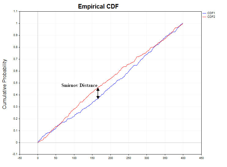
This statistic represents the exact upper bound (maximum) of the absolute value of the difference between the distribution functions. If the distribution law of a random variable does not change from sample to sample, then it is natural to expect low values of the Dn,m statistics. Excessively large values of this statistic, in turn, will testify against the null hypothesis of the data homogeneity. In actuality, to test statistical hypotheses, instead of the D statistic, a slightly modified statistic is calculated

lambda = D * ( sqrt(k) + 0,12 + 0,11/sqrt(k) ),

where k = (m*n/(m+n)). The distribution of the lambda statistic as k → ∞ in turn converges to the Kolmogorov distribution function:                                                  

Sometimes, a more simplified equation is used to calculate lambda when n equals m:

lambda = D *sqrt(n/2)

Next, having obtained certain statistical values, the homogeneity hypothesis is tested using sample data.

The statistical hypothesis is tested as follows:

• the null hypothesis H0 (the samples are homogeneous) and the alternative hypothesis H1 (the samples are heterogeneous) are formulated,

• the alpha significance level is adopted (the standard values of 0.1, 0.05 and 0.01 are usually used),

• u(alpha) critical value is calculated according to the Kolmogorov distribution (for example, if alpha is 0.05, u(alpha) is 1.3581),

• the sample value of the lambda statistic is calculated,

• if lambda < u(alpha), the null hypothesis is accepted,

• if lambda > u(alpha), the null hypothesis is rejected at the alpha significance level, as contradicting the observed data.

Another logical ending to this structure is also possible. Instead of the u(alpha) critical value, the probability PValue = 1 - K(lambda) is calculated and compared with the specified alpha significance level. If alpha ≥ PValue, the null hypothesis is rejected, since it is believed that an unlikely event occurred that is incompatible with the concept of randomness and therefore the samples should be recognized as different.

The figure here shows the derivative of the Kolmogorov distribution function, that is, the probability density function, calculated under the condition that the null hypothesis is true. If the Smirnov distance probability density function calculated for sample data differs from the Kolmogorov function, this may indicate data heterogeneity.

The two-sample Kolmogorov-Smirnov test should not be confused with the one-sample one. In the former, we compare two empirical distribution functions, while the latter compares the empirical and hypothetical distribution functions.

A very important point is that empirical distribution functions must be calculated using ungrouped observation data, since the Kolmogorov distribution function is calculated under this assumption. It is also important to emphasize that the two-sample Kolmogorov-Smirnov test does not depend on the specific type of distribution function. Since it can be difficult to draw a conclusion about whether the observed data belongs to one or another hypothetical type of distribution when analyzing financial time series, the value of this criterion for the analyst increases significantly. Without making any assumptions about the type of hypothetical distribution the observed data may belong to, we can test the homogeneity hypothesis solely on the basis of empirical distribution functions. For time series analysis, the Smirnov criterion can be considered as an indicator of process stationarity. After all, according to the definition of stationarity, a process is considered stationary when its probability distribution function does not change over time.

Simple calculation method explanation

Suppose that we have two large bags of marbles. One bag has marbles made in one country, while the other contains marbles made in another. Our task is to find out whether the marbles in both bags are the same or different.

1. Sorting marbles. First, we pour the balls out of both bags and arrange them according to size for each one - from the smallest to the largest.

2. Comparing marbles. Then we start looking at each marbles in the first bag and looking for a marble of the same size in the second bag. We measure how far apart similar marble are in two rows. In this context, "distance" means how far apart the marbles are in the rows when looking at their positions.
   
   Let's say we have a marbles from the first bag, which occupies the fifth position in the row. If a similarly sized marbles from the second bag is in the twentieth position in its row, then the distance between these two marbles will be equal to 15 positions (20 - 5 = 15). This number shows how far apart similar marbles are in two different bags (or two data samples).
   
   In the Kolmogorov-Smirnov statistical test, we compare such "distances" for all marbles and look for the maximum of them. If this maximum distance is greater than a certain value (which depends on the number of marbles in the bags), this may indicate that the marbles in the bags do differ in some properties.
   

3. Finding the biggest difference. We are looking for the place where the differences ("distances") between the marbles in the two rows are the greatest. For example, if in one place the marbles are very close in size, and in another they are very different, we mark this place.

4. Assessing the differences. If the largest distance between the marble is very large, this may mean that the marbles in the bags are indeed different. If all the marbles are fairly close to each other along the entire length of the row, they may indeed be from the same place.

Thus, if the differences between two rows of marbles are large, we say that the bags of marbles are different. If the differences are small, the marbles are most likely the same. This helps us understand whether marbles from two different places can be considered the same or not.

Data analysis using two-sample Kolmogorov-Smirnov test

Before proceeding to the analysis of D Smirnov distances, calculated on real quotes, first of all, we will examine how this statistic behaves on models of stationary processes, both with dependent and independent increments. For this purpose, I will generate 1000 samples (Samples) of time series with a given distribution function with a volume of 1440 data in each series. After that, I will calculate the D Smirnov distance between these samples, check in what percentage of cases the null hypothesis is rejected (H1/ Samples) and also construct an empirical probability density function of these distances in order to compare them with the Kolmogorov density function. The figure below shows the Smirnov distance series for a data sample of N = 1440, obtained from a normal and uniform distribution.       

                               
                               

For samples from a normal and uniform distribution, a false rejection of the homogeneity hypothesis occurs within the permissible error of the first type (alpha = 0.05), that is, in no more than 50 cases out of 1000 samples. H1/ Samples = 50/1000 = 0.05. Below are graphs of the sample probability density of Smirnov distances for normal and uniform distributions.

The X axis shows the lambda value.

As we can see, there is a complete matching of the sample distributions of the Smirnov distance for uniform and normal data samples and the Kolmogorov distribution, to which they should converge provided that the null hypothesis of homogeneity is true.

The normal and uniform distributions we just dealt with are examples of stationary independent processes. As a stationary but dependent process, I will take a discrete non-linear equation, often used as an example in the field of deterministic chaos - the logistic map:

Xn= R*Xn-1 *(1 – Xn-1), X0 = (0;1), R = 4

This is a one-dimensional non-linear dynamic system when the parameter R=4 exhibits chaotic behavior, almost indistinguishable from white noise. The autocorrelation function of the time series generated by this equation fluctuates around zero. However, there is a non-linear dependence in this process, and it would be interesting to check how this affects the distribution of Smirnov distances. This is not an idle question, since many believe that there are non-linear dependencies in financial data, so I included this equation in the analysis.

Of course, the analysis requires a model with linear dependencies, which may also be present in real data. Therefore, the second model of the stationary dependent process will be a linear autoregressive model of the first order:

ARt = 0.5 * ARt-1 + et

• et – a random variable with zero mean and unit variance, Gaussian white noise

The autoregressive process in this case is also a Gaussian process, albeit an already dependent one.

In processes with dependent increments, the situation with the rejection of the homogeneity hypothesis is slightly different. For the logistic mapping, there is a slight excess of the permissible value of the first type error of 0.058 (H1/ Samples= 58/1000), whereas for the first-order auto regression this error is already approximately 0.25 (H1/ Samples= 250/1000), that is five times greater than the permissible level under the null hypothesis.

We got a very interesting result. It turns out that according to the two-sample Kolmogorov-Smirnov test, we should recognize both the logistic mapping and AR(1) as inhomogeneous (non-stationary) processes. However, this is, of course, not the case. Why is that? It turns out that the probability density function of Smirnov distances for stationary distributions does not depend on the type of distribution of the process under study only if the observed data are statistically independent. Since both the logistic mapping and auto regression are processes with dependent increments, then in this case the probability density of the Smirnov distance will differ from the Kolmogorov distribution. This in turn means that the two-sample Kolmogorov-Smirnov test can be not only an indicator of heterogeneity (non-stationarity of the process) but also an indicator of the presence of data dependence (linear or non-linear).

Let's move on to analyzing real data. As an example, I took minute bars of the EURUSD currency pair and XAUUSD (gold).

For minute quotes, the percentage of deviation of the null hypothesis differs significantly from the stationary processes H1/ Samples = 466/1000 = 0.46 for XAUUSD and H1/ Samples = 640/1000 = 0.64 for EURUSD. For clarity, below is a graph of the sample probability density function of Smirnov distances for real data and dependent processes of auto regression and logistic mapping.

As we can see, a qualitatively different picture is observed here both for stationary dependent processes and for real EURUSD_M1 and XAUUSD_M1 quotes. The sample probability densities of Smirnov distances for these processes differ significantly from the Kolmogorov distribution. In this case, the processes of logistic mapping and first-order auto regression do not converge to the Kolmogorov distribution only due to the presence of statistical dependence in these data.

As for the prices of financial instruments, even after an attempt to reduce them to a stationary form using first differences, they are nevertheless remain non-stationary. A certain influence on such a large figure of deviation of the null hypothesis is most likely exerted by some dependencies that may be present in real quotes, as we saw from the analysis of stationary dependent processes. In my opinion, it is not possible to assess what share of the influence is due to dependencies in the data, and what share is due purely to the non-stationary component present in the time series of financial instruments. But the main influence still has to do with the heterogeneity of the data, as well as with the constant change in the probability distribution function of price increments.

In order to have a clear idea of what form the probability density of Smirnov distances for two heterogeneous samples can have, we will conduct another experiment, in which we will compare data from samples taken from two normal distributions belonging to different general populations. These distributions will differ in mathematical expectation and dispersion - N(0,1) vs N(0.1,1.2). It is obvious that two-sample Kolmogorov-Smirnov test should generally reject the null hypothesis of homogeneity. The mistake here would be to accept the null hypothesis when the alternative hypothesis is true. 

In this case, we have a percentage of rejection of the null hypothesis equal to 0.98 (H1/ Samples = 980/1000). The graph below shows the probability density functions of the Smirnov distance distribution for real quotes, the model of two non-uniform normal distributions and the Kolmogorov distribution.

As expected, in the model case of heterogeneity of two normal samples, the probability density function of Smirnov distances differs significantly from the Kolmogorov distribution homogeneous data should converge to. Note how sensitive the two-sample Kolmogorov-Smirnov test is to even relatively small changes in the distribution parameters. 

iSmirnovDistance indicator

Unlike the above analysis, iSmirnovDistance indicator performs calculation based solely on the amount of data contained in each of two adjacent trading days without allowing the data to overlap with other trading sessions. The indicator itself should be run on a daily timeframe, all calculations are made on 5-minute data of the same instrument. For currency quotes, this amounts to 287 data points per day. If on any of the days there are not enough quotes for calculations (I took 270 data as the limit), then the indicator values are set to zero.

Thus, at the beginning of each trading day, we receive the value of the Smirnov statistic calculated based on the values of the two previous trading days. This indicator can actually have only one parameter that can be optimized - the alpha significance level. In this version, I took the standard value equal to 0.05. The blue dotted line in the indicator window displays the Smirnov distance u(alpha) for the significance level alpha = 0.05, that is, for the null hypothesis. It is calculated using the above equation: lambda = D*sqrt(n/2). Knowing the critical value of lambda for the Kolmogorov distribution equal to 1.3581 (there are tables of the Kolmogorov distribution function) and the amount of data for the 5-minute timeframe equal to 287, we find the corresponding distance D = lambda / sqrt(n/2) = 1.3581/sqrt(287/2) = 0.1133. Exceeding this value by actual calculated values will indicate a qualitative change in the structure of the data distribution. The indicator values below the blue dotted line can be considered homogeneous.

It is worth saying that a timeframe the Smirnov distance is calculated on is also important. As we have seen, for minute data, there is significant non-stationarity of the series, while for the 5-minute timeframe, the series is more stationary and the homogeneity hypothesis is rejected much less often. This is partly due to the volume of data – 1440 for M1 versus 287 for M5. With a gradual increase in data from 287 to 1440, the rejection rate of the null hypothesis increases. However, the homogeneity hypothesis is more often rejected for M1 chart. 

Conclusion

This article was intended to answer a number of important questions regarding the analysis of stock exchange time series:

• The first question is whether a time series of logarithmic price increments can be considered stationary. In my opinion, a convincing answer has been received, confirmed by numerical calculations - no, it is not possible, at least for the minute timeframe. As for the five-minute timeframe, the series looks more stationary here compared to the minute one, but still demonstrates non-stationary behavior.

• The second question that this study attempts to answer is a logical continuation of the first one - what volume of data is needed to calculate a particular indicator? In my opinion, iSmirnovDistance indicator provides the following interpretation — for calculations, it is necessary to take the volume of data that falls within the time period between two deviations of the homogeneity null hypothesis. Until the null hypothesis is rejected, the amount of data to be analyzed gradually increases. After rejecting the null hypothesis, the previous data are discarded as obsolete and the data quantity calculation starts over. Thus, the volume of data to be analyzed is not a fixed value. This is a value that is constantly changing over time, as it should be, based on the nature of a non-stationary random process.