Neural networks made easy (Part 18): Association rules

Contents

• Introduction
• 1. Association rules
• 2. Apriori algorithm
• 3. FP-Growth algorithm
• Conclusion
• List of references

Introduction

The growth in the analyzed data volumes leads to a growth of interest in unsupervised learning methods. In the last few articles, we have already seen clustering and dimensionality reduction algorithms which belong to unsupervised learning methods. In this article, we continue studying unsupervised learning methods. This time, we will consider another type of problems which can be addressed within these methods: association rule mining. This problem type has originated from supermarket shopping marketing, where it was used to analyze market baskets with the purpose of finding the most frequently encountered product sets. Nowadays, algorithms solving these problems are widely used in various fields. We will look into how such algorithms can be used in trading.

1. Association rules

The problem of analyzing association rules belongs to Data Mining applied problems. Furthermore, it is one of the basic ones as it enables the identification of interesting relations between data in large databases.

This type of problem was first formulated and defined in retail shopping. The marketers were faced with the question of which business benefits can be derived from the analysis of a large database of transaction data registered by point-of-sale systems. Previously only total sales volumes were analyzed. The analysis of customer's receipts opened up new horizons, since it enabled the analysis of specific product sets purchased by customers.

The first algorithm was created by a group of developers from IBM back in 1993. This is when the main principles were formulated, which then formed the basis of a whole group of algorithms.

First of all, the rules detected by the algorithms must be frequently encountered. It means that they must not be random and must be repeated in the analyzed database no less than a certain number of times. It means that they must be confirmed. From the point of view of statistics, the sample of transactions containing such a rule should be representative. To meet this requirement, all algorithms used to determine association rules have a minimum support parameter MinSup, which indicates in fractions of "1" the ratio of the frequency of a rule occurrence to the total number of transactions in the analyzed sample.

According to the rules of combinatorics, if we have a set of 3 items: A, B and C, without taking into account the position of the elements, we can get 7 different sets containing from 1 to 3 of these items. As the number of items increases, the number of possible combinations also increases. Given the volume of databases, direct recalculation of frequency of each set becomes a rather resource-consuming task. Often such recalculation can be impossible. Therefore, the authors used the anti-monotonicity property.

If in the database, the A item is encountered with only one set of all possible, its frequency of occurrence will be equal to the frequency of A itself. If the number of sets encountered is greater, then their frequency can only be less, since the total number of their occurrences in the analyzed sample will be equal to the number of occurrences of A. Thus, if the frequency of occurrence of any item is less than MinSup, then the frequency of all possible variants of sets containing this item will be less than MinSup. So, it is enough for us to calculate the frequency of occurrence of each item in order to eliminate a significant part of random sets, which are of no practical value to us.

As you can see, association rules searching algorithms are very different from all those considered previously. Previously, we tried to make the most of all available data. In contrast, association rule mining algorithms immediately eliminate random (noise) items.

The second parameter used in all association rules algorithms is the minimum degree of confidence MinConf. It is also specified in fractions of 1. To explain this parameter, we should know that each rule consists of two parts: an antecedent and a consequent. Both the antecedent and the consequent can consist of either one item or a whole set of items. In the general case, the rule sounds as follows: if the antecedent is true, then quite often there will be a consequent.

Note that the probability of occurrence of the consequent after the occurrence of the antecedent is not 100%. While the minimum probability of the occurrence of the consequent is set by the MinConf parameter. When this parameter is met that the rule is considered valid and is saved into the array of rules. It is defined as the ratio of the rule execution frequency to the antecedent frequency.

2. Apriori algorithm

Probably one of the most famous algorithms for finding association rules is the Apriori algorithm, which was proposed by Rakesh Agrawal and Ramakrishnan Srikant in 1994. The algorithm is based on an iterative process of searching for the most frequent patterns in the database. After that, rules are extracted from the selected patterns.

To better understand it, let's look at the operation of the algorithm on a small example of 10 transactions with 5 items.

Transaction ID	Contents
T1	BCDE
T2	BCD
T3	B
T4	BCD
T5	D
T6	ACD
T7	BCDE
T8	BCE
T9	CDE
T10	AD

Let's introduce into the problem the constants of the minimum support 0.3 and the minimum confidence 0.7 (30% and 70%, respectively).

Please note that all association rule algorithms work with binary arrays. Therefore, to get started, let us present the above data as a binary table.

Transaction ID	A	B	C	D	E
T1	0	1	1	1	1
T2	0	1	1	1	0
T3	0	1	0	0	0
T4	0	1	1	1	0
T5	0	0	0	1	0
T6	1	0	1	1	0
T7	0	1	1	1	1
T8	0	1	1	1	0
T9	0	0	1	1	1
T10	1	0	0	1	0

Based on this table, it is easy to calculate that item A occurs only two times and its support is equal to 0.2 or 20%. Similarly, let's calculate support for other items: B — 0.6, C — 0.7, D — 0.8, E — 0.4. As you can see, only A does not meet the minimum support requirement. So, we exclude it from further processing according to the anti-monotonicity property.

From the remaining elements, we create candidates for frequently occurring patterns. We have determined frequently occurring items in the previous step. According to the algorithm, let us determine candidates into sets of two items: BC, BD, BE, CD, CE, DE.

Now, we need to process the entire database and determine the support for each of the selected candidates.

Transaction ID	BC	BD	BE	CD	CE	DE
T1	1	1	1	1	1	1
T2	1	1	0	1	0	0
T3	0	0	0	0	0	0
T4	1	1	0	1	0	0
T5	0	0	0	0	0	0
T6	0	0	0	1	0	0
T7	1	1	1	1	1	1
T8	1	0	1	0	1	0
T9	0	0	0	1	1	1
T10	0	0	0	0	0	0

This time the support of all our candidates meets satisfies the minimum support condition: BC — 0.5, BD — 0.4, BE — 0.3, CD — 0.6, CE — 0.4, DE — 0.3. But this does not always happen. When solving practical problems, some candidates are more likely to be eliminated.

Next, we continue the iterative process. This time let's create candidate sets of three items. To do this, we take the frequent patterns selected at the previous iteration and combine pairs that differ in only one element. We can determine 4 candidates: BCD, BCE, BDE, CDE.

According to the Apriori algorithm, we have to go through the entire database again in order to determine the support for all new candidates.

Transaction ID	BCD	BCE	BDE	CDE
T1	1	1	1	1
T2	1	0	0	0
T3	0	0	0	0
T4	1	0	0	0
T5	0	0	0	0
T6	0	0	0	0
T7	1	1	1	1
T8	0	1	0	0
T9	0	0	0	1
T10	0	0	0	0

As a result, we obtain the following support values for our candidates: BCD — 0.4, BCE — 0.3, BDE — 0.2, CDE — 0.3. In this iteration, support for the BDE itemset does not satisfy the minimum support requirement and we therefore exclude it. Other candidates are considered as frequent patterns.

At the next iteration, we compile candidate sets of 4 items. Based on the patterns selected at the previous iteration, we can make only one candidate BCDE. But before going calculating the support for this candidate, let's pay attention to its component BDE. This candidate was removed after the previous iteration as it support was only 0.2, while the minimum support requirement is 0.3. Therefore, according to the anti-monotonicity rule, the BCDE candidate cannot have support greater than 0.2. But this is below the minimum support.

Since we do not have any other candidates, we stop the process of searching for frequent pattens and move on to the next subprocess — determining rules based on the selected frequent patterns. To do this, we divide the selected patterns into an antecedent and consequent. After that, we can determine the confidence level for each rule and compare it to the minimum required confidence level.

We will build the rules sequentially, for each item from the set. Since at the very first stage we eliminated all patterns with A (its support is below MinSup), let's start determining the rules with B.

From the selected patterns, let's determine all those containing the analyzed item. Extract item B from the patterns to be used as a consequent, while the remaining part will be the antecedent. We will also determine the confidence for each created rule.

The rule confidence degree shows with what probability a consequent appears when the antecedent is formed. To determine it, we do not need to re-iterate the entire database. We simply need to divide the support for the full pattern to the support of the antecedent which has previously been calculated at the frequent pattern selection stage.

Pattern	Antecedent	Support	Rule
BC (0.5)	C (0.7)	0.71	C -> B
BD (0.4)	D (0.8)	0.50	D -> B
BE (0.3)	E (0.4)	0.75	E -> B
BCD (0.4)	CD (0.6)	0.67	CD -> B
BCE (0.3)	CE (0.4)	0.75	CE -> B

Rules D -> B and CD -> B do not meet the minimum support requirement of 0.7 and we therefore exclude them.

Determine other rules in a similar way.

Pattern	Antecedent	Support	Rule
BC (0.5)	B (0.6)	0.83	B -> C
CD (0.6)	D (0.8)	0.75	D -> C
CE (0.4)	E (0.4)	1.00	E -> C
BCD (0.4)	BD (0.4)	1.00	BD -> C
BCE (0.3)	BE (0.3)	1.00	BE -> C
CDE (0.3)	DE (0.3)	1.00	DE -> C
CD (0.6)	C (0.7)	0.86	C -> D
DE (0.3)	E (0.4)	0.75	E -> D
BCD (0.4)	BC (0.5)	0.80	BC -> D
CDE (0.3)	CE (0.4)	0.75	CE -> D

We have seen one of the most well-known algorithms for association rule mining Apriori. However, despite its simplicity and popularity, it is rarely used in practice. This is because the bottleneck of the considered method is the multiple iteration through the database required to evaluate the support of candidates for frequent patterns. As the volume of databases under analysis grows, this becomes more and more of a problem. This problem is efficiently addressed in the next algorithm. It only requires to iterations for a database of any volume and with any number of analyzed items.

3. FP-Growth algorithm

Let us consider the solution of the problems described above using an example of one of the fastest algorithms for finding association rules: FP-Growth (Frequent Pattern - Growth). Due to the algorithm construction specifics, a complete iteration of all elements of the training sample is performed only 2 times in the process of its execution. The algorithm does not call the training sample except for these two times.

Similar to the earlier considered association rule mining algorithm, FP-Growth can be conditionally divided into two subproblems:

1. Finding frequently occurring patterns. In this example this stage is referred to as the building of an FP tree.
2. Determining the rules.

The algorithm starts by eliminating random items. To do this, like in the previous algorithm, we perform the first pass for the entire training set and calculate the support for each item. After that delete all items with the frequency less than MinSup.

The remaining items are arranged in descending order of their supports. The above example results in the following series:

D (0.8) -> C (0.7) -> B (0.6) -> E(0.4) 

Next, we will grow the FP-tree. To do this, implement the second pass over the training sample. In each transaction, we only take frequent items arranged in descending order of supports and build a path in the tree. Thus, the node with the highest support will be in the tree root, while that with the lowest one will be a leaf. We also create a counter for each node. At the first iteration, we set the counter value equal to 1 (or 1/N, where N is the size of the training sample).

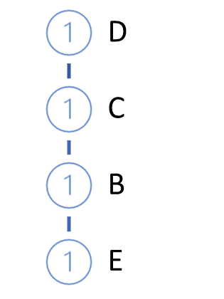
Then we take the next transaction from the database. Build a path for it in the same way. Add it to our tree. To do this, starting from the tree root, we check the path with already existing branches. When repeating the path from the root, we simply increase the counter of existing nodes. For the new part, create a branch.

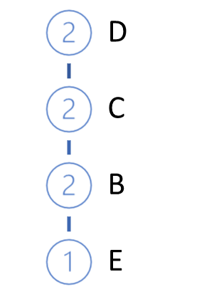
The cycle of iterations is repeated until the complete iteration of the entire training set. For the above example, we will get the following FP-tree.

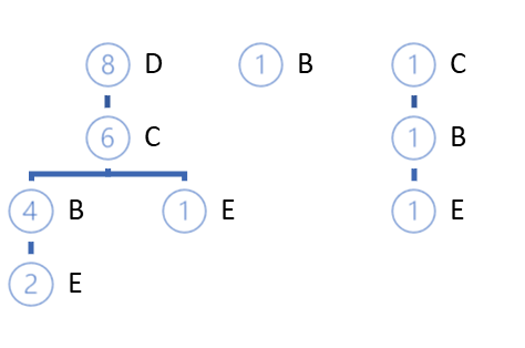
With a high degree of probability, we can find the paths that differ from the root itself. There are two options possible:

• Building a forest
• Creating a certain root node that will unite the entire selection.

Obviously, at the beginning of the FP tree growing process, new nodes will be created for the most part. But in the process of moving along the training sample, we will come to an increase in the counters of existing nodes without creating new branches. The specific feature of this algorithm is that in the process of building a tree, we can compress the training sample to such sizes that we can easily operate within the computer's RAM without accessing the database.

Further work related to the definition of rules is performed only with the FP tree, without using the original database.

Rules are constructed for all items in ascending order of their support.

At the first stage we already eliminated all items with a frequency less than the specified one, and now our tree contains only frequently occurring items. In addition, when constructing the tree, we sorted the items in descending order. It means that the items with the lowest support are the leaves.

So, to determine the rules starting with the lowest support items, we move from leaves to the root. Here we can trace the not yet explicit causal relationship. The algorithm assumes that items with less support appear as a result of a combination of features with more support.

But lets' back to our rule definition algorithm. Take lowest support items and determine all paths in the FP tree that lead to this item. When selecting the paths, we first pay attention to the frequency of occurrence of the desired item in the formation of the pattern from the path items. The path selection criterion is the ratio of the item support to the support of the previous node. The ratio must not be less than the minimum confidence of the rule.

In the above example, the lowest support is shown by E. Three paths in the FP-trees lead to it: DCBE (0.2), DCE (0.1), CBE(0.1). None of the paths meets the minimum support requirement. Two of them do not meet the minimum confidence requirement. Therefore, we cannot create a rule for E. Note that this is confirmed by the results obtained via the Apriori algorithm. 

Delete E leaves from the tree and get the following FP-tree view.

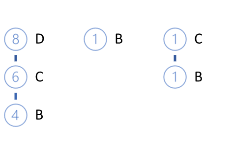
The next element to be analyzed is B. It has the lowest support among those left. It has three paths: DCB (0.4), B (0.1), CB (0.1).

In the selected support paths, each item preceding the analyzed one is assigned the support of the analyzed item in the given path.

Based on the selected paths, we form a list of participating items and determine the support of each of them. Note that support is determined as the ratio of the number of item occurrences in the selected paths to the total number of records in the original training dataset. Thus, the new support of each item cannot exceed the initial item support or the support of the analyzed item (for which the rules are being determined).

Again, we also remove items with less than minimal support. Arrange the remaining items in descending order of support.

In this example, we have C (0.5), D (0.4).

Note that since we have calculated item support only using the selected paths, the results may considerably differ from the initial ones. As a result of this factor, some items can be eliminated and their order in the new hierarchy will change.

Further, in accordance with the new hierarchy, we build a new private tree using the selected paths. The tree construction algorithm does not differ from the FP-tree construction.

The branches of the constructed private tree will be the antecedent of the rules, the consequent of which will be our analyzed item.

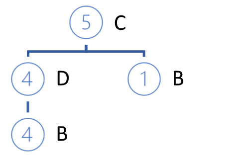
After constructing the private tree, we remove the nodes of the analyzed item from the original FP tree. The trick is that we analyzed the item with minimal support. This means that all nodes containing this items are the leaves of the FP-tree. Therefore, their removal will not affect the paths of other items (a little higher we mentioned a causal relationship).

In addition, by gradually removing the analyzed features, we gradually reduce our FP tree. Thereby we reduce the amount of data for the further search in the analysis of other items. This affects the overall performance of the algorithm.

Similarly, we build rules for each item in the original hierarchy of the FP trees.

Note that we can only build rules for items for which there is at least one root node in the FP tree. We cannot create rules for root items, as we have nothing to use as an antecedent. Of course, except for the visit of a potential customer to the supermarket. If the customer has come to the supermarket, they will buy something. Most likely this will be one of the best-selling items. But this is beyond the scope of the algorithm under consideration.

Conclusion

In this article, we considered another type of problems solved by unsupervised learning methods: association rule mining. We have discussed two association rule mining algorithms: Apriori and FP-Growth. But there are many other algorithms. Unfortunately, I can't cover the whole topic within one article. Furthermore, it only provides theoretical aspects. In the next article, we will consider the practical construction of an association rule mining algorithm using MQL5. We will also evaluate its efficiency applied for a practical trading task.

List of references

1. Neural networks made easy (Part 14): Data clustering
2. Neural networks made easy (Part 15): Data clustering using MQL5
3. Neural networks made easy (Part 16): Practical use of clustering
4. Neural networks made easy (Part 17): Dimensionality reduction
5. Fast Algorithms for Mining Association Rules
6. Mining Frequent Patterns without Candidate Generation