
Neural networks made easy (Part 89): Frequency Enhanced Decomposition Transformer (FEDformer)

Introduction
Long-term forecasting of time series is a long-standing problem in solving various applied problems. Transformer-based models show promising results. However, high computational complexity and memory requirements make it difficult to use the Transformer for modeling long sequences. This has given rise to numerous studies devoted to reducing computational costs of the Transformer algorithm.
Despite the progress made by Transformer-based time series forecasting methods based, in some cases they fail to capture the common features of the time series distribution. The authors of the paper "FEDformer: Frequency Enhanced Decomposed Transformer for Long-term Series Forecasting" have made an attempt to solve this problem. They compare the actual data of a time series with its predicted values obtained from the vanilla Transformer. Below is a screenshot from that paper.
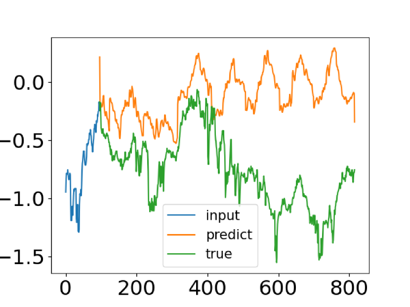
You can see that the distribution of the forecast time series is very different from the true one. The discrepancy between expected and predicted values can be explained by the point attention in the Transformer. Since the forecast for each time step is made individually and independently, it is likely that the model cannot preserve the global properties and statistics of the time series as a whole. To solve this problem, the authors of the article exploit two ideas.
The first is to use the seasonal trend decomposition approach, which is widely used in time series analysis. The authors of the paper present a special model architecture that effectively approximates the distribution of forecasts to the true one.
The second idea is to implement Fourier analysis into the Transformer algorithm. Instead of applying the Transformer to the time measurement of the sequence, we can analyze its frequency features. This helps the Transformer better capture the global properties of time series.
The combination of the proposed ideas is implemented in the Frequency Enhanced Decomposition Transformer model, FEDformer.
One of the most important questions related to FEDformer is which subset of frequency components should be used in Fourier analysis to represent the time series. In such analyses, low-frequency components are most often retained and high-frequency components are discarded. However, this may not be appropriate for time series forecasting since some changes in time series trends are associated with important events. This part of the information can be lost by simply removing all high-frequency components of the signal. The authors of the method accept the fact that time series usually have unknown sparse representations based on the Fourier basis. Their theoretical analysis showed that a randomly selected subset of frequency components, including both low and high ones, provides a better representation of the time series. This observation has been confirmed by extensive empirical research.
In addition to improving the efficiency of long-term forecasting, the combination of the Transformer with frequency analysis can reduce computational costs from quadratic to linear complexity.
The authors of the paper summarize their achievements as follows:
1. They propose a signal decomposition architecture Transformer with improved frequency response and the use of experts for seasonal-trend decomposition in order to better capture global properties of time series.
2. They propose Fourier enhanced blocks and Wavelet enhanced blocks in the Transformer architecture, that allow the capturing of important structures in time series by studying frequency features. They serve as substitution for both self-attention and cross-attention blocks.
3. By randomly selecting a fixed number of Fourier components, the proposed model achieves linear computational complexity and memory cost. The effectiveness of this selection method has been proved both theoretically and empirically.
4. Experiments conducted on six baseline datasets in different domains show that the proposed model improves the performance of state-of-the-art methods by 14.8% and 22.6% for multivariate and univariate forecasting, respectively.
1. The FEDformer Algorithm
The authors of the method presented 2 versions of the FEDformer model. One uses the Fourier basis to analyze the frequency features of a time series. The second one is based on the use of wavelets, which allow combining analysis both in terms of time and in the area of frequency features.
Forecasting long-term time series is a sequence-to-sequence problem. Let us denote the size of the sequence of initial data as I and the predicted sequence as O. Let D represent the size of the vector describing one state of the series. Then we feed a tensor of size I*D into the Encoder, and the Decoder is fed the matrix (I/2+O)*D.
As mentioned above, the authors of the method improve the Transformer architecture by introducing into it the analysis of seasonal-trend decomposition and distribution. The updated Transformer features a deep decomposition architecture and includes a frequency response analysis unit (FEB), frequency enhanced attention block (FEA), Mixture Of Experts decomposition blocks (MOEDecomp).
The FEDformer Encoder uses a multi-level structure similar to the Transformer Encoder. A separate block of it can be represented by the following mathematical expressions:
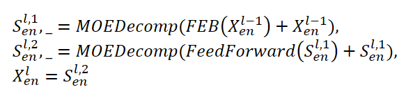
Here Sen represents the seasonal component extracted from the original data in the MOEDecomp decomposition block.
For the FEB module, the authors of the method propose two different versions (FEB-f and FEB-w), which are implemented using the discrete Fourier transform mechanism (DFT) and discrete Wavelet transform (DWT), respectively. In this implementation, they replace the Self-Attention block.
The Decoder also uses a multi-level structure, just like the Encoder. But the architecture of its constituent blocks is much broader and is described by the formulas:
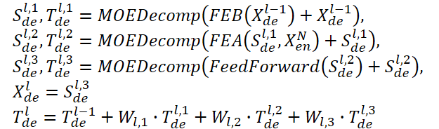
Sde and Tde represent the seasonal and trend component after the MOEDecomp decomposition block. Wl acts as a projection for the extracted trend. Like FEB, FEA has two different versions (FEA-f and FEA-w), which are implemented through DFT and DWT projection, respectively. FEA is implemented with attention design and replaces the cross attention block of the vanilla Transformer.
The final forecast is the sum of the two refined decomposed components. The seasonal component is projected using the WS matrix to the target measurement.
![]()
The proposed FEDformer model uses the discrete Fourier transform (DFT), which allows the analyzed sequence to be decomposed into its constituent harmonics (sinusoidal components). To improve the efficiency of the model, the authors of FEDformer use the fast Fourier transform (FFT).
As mentioned earlier, the method uses a random subset of the Fourier basis, and the scale of the subset is limited by a scalar. Selecting a mode index before DFT and inverse DFT (IDFT) operations allows you to further adjust the complexity of calculations.
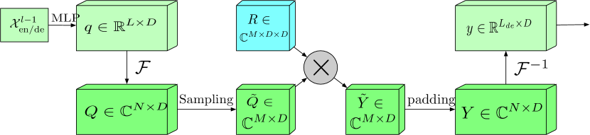
Extended frequency range block with Fourier transform (FEB-f) is used in both the Encoder and the Decoder. Source data of the FEB-f block is first linearly projected and then transformed from the time domain to frequency responses. Mharmonics are randomly sampled from the obtained frequency characteristics. After that, the selected frequency features are multiplied by the matrix of the parameterized kernel, which is initialized with random parameters and adjusted during the model training process. The result is zero-padded to the full frequency response dimensions before performing the inverse Fourier transform, which returns the analyzed sequence to the time domain. The original visualization of the FEB-f block provided by the paper authors is presented below.
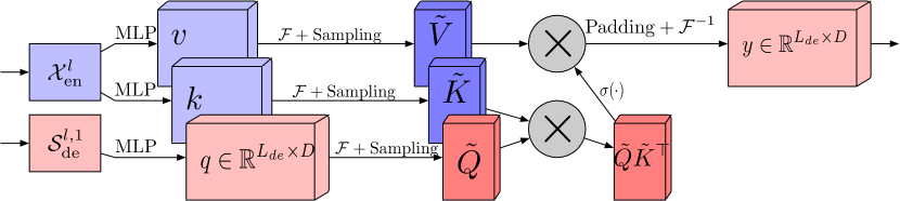
The frequency response attention block using the discrete Fourier transform (FEA-f) applies the canonical Transformer approach with a small addition. The source data is transformed into Query, Key and Value representations. With cross attention, Query come from the Decoder, while Key and Value come from Encoder. However, in FEA-f, we transform Query, Key and Value using the Fourier transform and perform a similar canonical attention mechanism in the frequency area. Here, as in the FEB-f block, for analysis we randomly sample M harmonics. The result of the attention operation is padded with zeros to the size of the original sequence, and the inverse Fourier transform is performed. The FEA-f structure in the author's visualization is shown below.
While the Fourier transform creates a frequency domain representation of a signal, the wavelet transform allows the signal to be represented in both the frequency and time domains, providing efficient access to localized information about the original signal. The multiwavelet transform combines the advantages of orthogonal polynomials and wavelets. A multiwavelet representation of a signal can be obtained by tensor product of a multiscale and multiwavelet basis. Note that bases at different scales are related by a tensor product. Authors of the FEDformer method adapt a non-standard wavelet representation to reduce the complexity of the model.
The FEB-w architecture differs from FEB-f in the recursive mechanism: the original data is recursively decomposed into 3 parts, and each of them is processed individually. For wavelet decomposition, the authors of the method propose a fixed matrix of the Legendre wavelet basis decomposition. Three FEB-f modules are used to process the resulting high-frequency part, low-frequency part and the remaining part of the wavelet decomposition, respectively. Each iteration creates a processed high-frequency tensor, a processed low-frequency tensor, and a raw low-frequency tensor. This is a top-down approach and the decomposition step gaps the signal by a factor of 1/2. Three sets of FEB-f blocks are used together during different decomposition iterations. Regarding wavelet reconstruction, the authors of the method also recursively create the output tensor.
FEA-w contains a decomposition stage and a reconstruction stage, similar to FEB-w. Here are the authors of FEDformer leave the reconstruction stage unchanged. The only difference is the decomposition stage. The use the same matrixto decompose the signal into the Query, Key and Value entities. As shown above, the FEB-w block contains three FEB-f blocks for signal processing. FEB-f can be considered as a replacement for the Self-Attention mechanism. The authors of the method use a simple method to create frequency-enhancing cross-attention using wavelet decomposition, replacing each FEB-f with an FEA-f module. In addition, the add one more FEA-f module to process the coarsest residues.
Due to the often observed complex periodic pattern combined with a trend component, trend extraction may be difficult in real data when merging fixed-window averages. To overcome this problem, the developed the Mixture of Experts decomposition block (MOEDecomp). It contains a set of filters of different average sizes to extract multiple trend components from the original signal, and a set of data-dependent weights to combine them into the resulting trend.
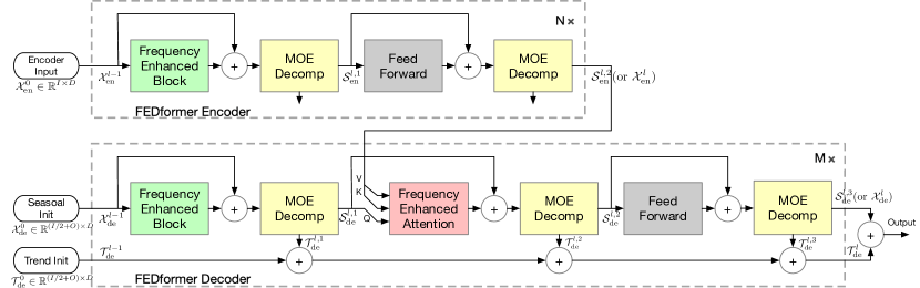
The complete algorithm of the FEDformer method is presented in the authors' original visualization below.
2. Implementing in MQL5
We have considered the theoretical aspects of the proposed FEDformer method. I must admit that our implementation will be far from the original. We will use the proposed approaches, but will not fully implement the proposed algorithm. There are several of my personal convictions about this.
First, we need to decide which base we will use: DFT or DWT. The question is quite complex and ambiguous. But we will do it much more simply. Let us turn to the method testing results which are presented in the original paper.

Pay attention to the "Exchange" column. We will not go into detail on what data exactly the model was tested, but there is a clear superiority of the model using DWT. Perhaps, as there is no clear periodicity in the input data, DFT is unable to determine the trend change moment. Actually, the method ignores the time component of the input data. DWT, which analyzes the signal in both dimensions, is able to provide more accurate predictive data. I think in this situation the choice of DWT is obvious.
2.1 Implementing DWT
We have decided on the implementation basis. Let's now start by implementing the wavelet decomposition in our library. For this, we create a new object CNeuronLegendreWavelets.
Let's think a little about the architecture of the object being created. As already mentioned above, for wavelet decomposition, the authors of the method propose to use a fixed matrix of the Legendre wavelet basis decomposition. In other words, to decompose a signal, we only need to multiply the signal vector by the wavelet basis matrix.
In our input data sequence, we have to analyze several parallel signals of a multimodal time series. For each unitary time series, we will use the same basis matrix.
This process is very similar to convolution with multiple filters. But in this case, the role of the filter matrix is performed by the wavelet basis matrix. Logically, we can create a new object as a successor to our convolutional layer. With a thoughtful approach, we can make the most of inherited methods by overriding just a couple of them.
class CNeuronLegendreWavelets :  public CNeuronConvOCL
  {
protected:
   virtual bool      updateInputWeights(CNeuronBaseOCL *NeuronOCL)   { return true; }

public:
                     CNeuronLegendreWavelets(void) {};
                    ~CNeuronLegendreWavelets(void) {};
   virtual bool      Init(uint numOutputs, uint myIndex, COpenCLMy *open_cl,
                          uint window, uint step, uint units_count,
                          ENUM_OPTIMIZATION optimization_type, uint batch);
   //---
   virtual int       Type(void)   const   {  return defNeuronLegendreWavelets;   }
  };
In the above structure of the new class CNeuronLegendreWavelets, you can see only 3 overridden methods, one of which is the class identifier Type returning a predefined constant.
The second point, which was already mentioned above, is that we use a fixed matrix of basis wavelets. Therefore, there will be no trainable parameters in our class, and the updateInputWeights method is redefined by a "stub".
In fact, we only have to work with the class object initialization method Init. In the new method, we do not declare any local variables or objects. In the initialization method, we only have to fill in the matrix of basis wavelets.
The authors of the method propose using Legendre polynomials as wavelets. I have selected 9 such polynomials, the visualization of them is presented below.

As you can see, with the polynomials presented on the graph, we can describe a fairly wide range of frequencies.
Also note that the range of acceptable values of the presented polynomials is [0, 1]. This is quite convenient. We define the window length of the analyzed sequence as 1. Then we divide the range by the number of elements in the sequence. In this way we define the time step between two adjacent elements of the sequence, which we initially form with a fixed step. Here the timeframe of the collected initial data does not matter. We analyze the frequency features of the signal within the visible window of the original sequence.
And here we are faced with the problem of determining the number of elements in a sequence at the model design stage. Before creating the base matrix, we need to specify its dimensions. At this stage we only have the number of filters we have selected. We will know the window size of the analyzed sequence only when initializing the model. In fact, we have 2 options to get out of this situation:
- We can determine strict dimensions of the matrix of basis wavelets and fill in its values immediately. And using a trainable convolutional layer before the matrix will allow us to work with any size of the original sequence.
- Create a universal algorithm for filling the matrix of basis wavelets at the stage of model initialization for any size of initial data.
The first option allows us to fill the matrix with fixed values in any available way. We can even find the coefficients of the basic wavelets we are interested in on the web. But how do we determine this "golden mean" between accuracy and performance? Moreover, the requirements for forecast accuracy can vary greatly in different tasks.
In my opinion, the second option looks more suitable for our purposes. To implement it, we will create formulas for the selected polynomials as macro substitutions. Below are some of them (the complete list is available in the attachment):
#define Legendre4(x)    (70*pow(x,4) - 140*pow(x,3) + 90*pow(x,2) - 20*x + 1)
#define Legendre6(x)    (924*pow(x,6) - 2772*pow(x,5) + 3150*pow(x,4) - 1680*pow(x,3) + \
                         420*pow(x,2) - 42*x + 1)
#define Legendre8(x)    (12870*pow(x,8) - 51480*pow(x,7) + 84084*pow(x,6) - 72072*pow(x,5) + \
                         34650*pow(x,4) - 9240*pow(x,3) + 1260*pow(x,2) - 72*x + 1)
Using these macro substitutions, we can obtain the value of the polynomial for any discrete value. After completing the preparatory work, we can proceed to the description of the algorithm for initializing an object of our new class CNeuronLegendreWavelets::Init.
In the parameters to the method we pass the key parameters of the object architecture:
bool CNeuronLegendreWavelets::Init(uint numOutputs, uint myIndex, COpenCLMy *open_cl,
                                   uint window, uint step, uint units_count,
                                   ENUM_OPTIMIZATION optimization_type, uint batch)
  {
   if(!CNeuronConvOCL::Init(numOutputs, myIndex, open_cl, window, step, 9, units_count,
                            optimization_type, batch))
      return false;
In the body of the method, we first call the same method of the parent class.
Note that in the parameters of the initialization method of the new class we receive only the window size of the sequence being analyzed and the number of elements in the sequence. When calling the relevant method of the parent class, we need to add the window step and the number of filters. As we have decided earlier regarding the number of filter, we will have 9 of them. As for the the step of the analyzed window, it will be equal to the analyzed window.
After the method of the parent class has been successfully initialized, our convolution parameter matrix is filled with random values. But we need to fill it with the basic parameters of the wavelet. So, we first fill the weight matrix with zero values. This is a very important point, since we need to reset the specified bias parameters.
WeightsConv.BufferInit(WeightsConv.Total(), 0);
Then in the loop we fill the matrix with the values of the basis wavelets:
   for(uint i = 0; i < iWindow; i++)
     {
      uint shift = i;
      float k = float(i) / iWindow;
      if(!WeightsConv.Update(shift, Legendre4(k)))
         return false;
      shift += iWindow + 1;
      if(!WeightsConv.Update(shift, Legendre6(k)))
         return false;
      shift += iWindow + 1;
      if(!WeightsConv.Update(shift, Legendre8(k)))
         return false;
      shift += iWindow + 1;
      if(!WeightsConv.Update(shift, Legendre10(k)))
         return false;
      shift += iWindow + 1;
      if(!WeightsConv.Update(shift, Legendre12(k)))
         return false;
      shift += iWindow + 1;
      if(!WeightsConv.Update(shift, Legendre16(k)))
         return false;
      shift += iWindow + 1;
      if(!WeightsConv.Update(shift, Legendre18(k)))
         return false;
      shift += iWindow + 1;
      if(!WeightsConv.Update(shift, Legendre20(k)))
         return false;
     }
Transfer the filled matrix into the OpenCL context memory:
   if(!!OpenCL)
      if(!WeightsConv.BufferWrite())
         return false;
//---
   return true;
  }
Complete the method execution.
In this implementation, we inherited all the remaining functionality necessary for the correct operation of the object from the parent class. Therefore, we finish working on this class and move on.
2.2 FED-w Block
The next stage can be considered as moving up a notch. We will create our own vision of the FED-w block. Its functionality is implemented in the CNeuronFEDW class. The structure of this class is presented below.
class CNeuronFEDW : public CNeuronBaseOCL
  {
protected:
   //---
   uint                    iWindow;
   uint                    iCount;
   //---
   CNeuronLegendreWavelets cWavlets;
   CNeuronBatchNormOCL     cNorm;
   CNeuronSoftMaxOCL       cSoftMax;
   CNeuronConvOCL          cFF[2];
   CNeuronBaseOCL          cReconstruct;
   //---
   virtual bool      feedForward(CNeuronBaseOCL *NeuronOCL);
   virtual bool      updateInputWeights(CNeuronBaseOCL *NeuronOCL);
   virtual bool      calcInputGradients(CNeuronBaseOCL *NeuronOCL);
   //---
   virtual bool      Reconsruct(CBufferFloat* inputs, CBufferFloat *outputs);

public:
                     CNeuronFEDW(void) {};
                    ~CNeuronFEDW(void) {};
   //---
   virtual bool      Init(uint numOutputs, uint myIndex, COpenCLMy *open_cl,
                          uint window, uint count,
                          ENUM_OPTIMIZATION optimization_type, uint batch);
   //---
   virtual bool      Save(int const file_handle);
   virtual bool      Load(int const file_handle);
   //---
   virtual int       Type(void)        const                      {  return defNeuronFEDW; }
   virtual void      SetOpenCL(COpenCLMy *obj);
   //---
   virtual bool      WeightsUpdate(CNeuronBaseOCL *source, float tau);
  };
You can see that this class has a more complex architecture compared to the previous one. It declares 2 local variables to store key parameters. Also we declare here a whole series of internal objects. We will see their purpose during the implementation process. All objects are declared statically. This allows us to leave the class constructor and destructor "empty".
Initialization of all nested objects is performed in the CNeuronFEDW::Init method. Object architecture parameters are passed to the method. These, among others, include the fundamental parameters of the size of the visible data window (window) and the number of analyzed unitary sequences (count).
bool CNeuronFEDW::Init(uint numOutputs, uint myIndex, COpenCLMy *open_cl,
                       uint window, uint count,
                       ENUM_OPTIMIZATION optimization_type, uint batch)
  {
   if(!CNeuronBaseOCL::Init(numOutputs, myIndex, open_cl, window * count,
                            optimization_type, batch))
      return false;
In the body of the method, we first call the relevant method of the parent class. After that, we save the architecture parameters of the initialized object in local variables:
   iWindow = window;
   iCount = count;
Then we initialize the internal objects in the same order in which they will be used.
Initially, we plan to extract frequency characteristics from the received raw data. For this, we use an instance of the above created CNeuronLegendreWavelets class:
   if(!cWavlets.Init(0, 0, OpenCL, iWindow, iWindow, iCount, optimization, iBatch))
      return false;
   cWavlets.SetActivationFunction(None);
The FED-w block we are creating is greatly simplified compared to the method proposed by the authors. I decided not to use DFT blocks. It seems to me that the frequency analysis in isolation from the time component can work against us and reduce the quality of forecasts. Therefore, there is a question regarding the appropriateness of using DFT. But this is my personal opinion, and it might be wrong.
Moreover, the elimination of a rather labor-intensive FFT process will significantly reduce the cost of computing resources during the training and operation of the model.
With that said, I decided to go towards the improvement of the model performance while accepting the risks of possible deterioration in forecasting quality.
I first normalize the data obtained after wavelet decomposition using a batch normalization layer:
   if(!cNorm.Init(0, 1, OpenCL, 9 * iCount, 1000,optimization))
      return false;
   cNorm.SetActivationFunction(None);
And then I evaluate the share of each of the filters used. To do this, I translate the obtained data into the probability subspace using the SoftMax function.
   if(!cSoftMax.Init(0, 1, OpenCL, 9 * iCount, optimization, iBatch))
      return false;
   cSoftMax.SetHeads(iCount);
   cSoftMax.SetActivationFunction(None);
Please note that we evaluate each unitary channel separately.
We then reconstruct the original time series from the probabilistic representation by inversely convolving it with our wavelet basis matrix. The result is saved in the created nested base layer:
   if(!cReconstruct.Init(0, 2, OpenCL, iWindow, optimization, iBatch))
      return false;
   cReconstruct.SetActivationFunction(None);
It can be seen that the above operations form a kind of circle: time series → wavelet decomposition → normalization → probability representation → time series. But what we get at the output is a fairly smoothed representation of the input time series, which we passed through a kind of digital filter. As a result, we get quite efficient data filtering with a minimum of trainable parameters that are present only in the batch normalization layer. This block replaces Self-Attention in our implementation.
The important thing to note here is that we are essentially replacing the model's trainable parameters with pre-defined wavelets. This makes our model more understandable, as opposed to the "black box" of trainable parameters, but less flexible. This also places an additional burden on the model architect in terms of finding optimal wavelets to solve the given problem. That is why I put wavelet polynomials into a separate block of macro substitutions. This approach will allow us to experiment with different wavelets and find the optimal ones.
But let's return to our class initialization method. The digital filter block is followed by the FeedForward block that is quite common for the Transformer architecture. Here we use an unchanged 2-layer MLP with LReLU between layers. As before, to implement independent channel processing, we use convolutional layer objects:
   if(!cFF[0].Init(0, 3, OpenCL, iWindow, iWindow, 4 * iWindow, iCount, optimization, iBatch))
      return false;
   cFF[0].SetActivationFunction(LReLU);
   if(!cFF[1].Init(0, 4, OpenCL, 4 * iWindow, 4 * iWindow, iWindow, iCount, optimization, iBatch))
      return false;
   SetActivationFunction(None);
At the end of the initialization method, we organize the replacement of the error gradient buffer in order to minimize unnecessary data copying operations:
   if(Gradient != cFF[1].getGradient())
      SetGradient(cFF[1].getGradient());
//---
   return true;
  }
After completing the work on initializing our object, we move on to implementing a feed-forward pass of the proposed model. From the above description of the planned process, it is worth highlighting the inverse convolution of the obtained probabilities into a time series.
"Inverse convolution" sounds like something new in our implementation. However, we have already implemented this process a long time ago. Using inverse convolution we propagate the error gradient in the convolutional layer. But now we need to implement the specified process within the feed-forward pass.
The difficulty is that all methods of our classes work with a fixed list of data buffers. This allows us to not think about the data buffers used during the process of creating models. We just need to provide a pointer to the object, while all data buffers are already written in the method. The "downside" is that we cannot use the backpropagation method to implement the algorithm within the feed-forward pass. However, we can create a new method in which we will use the previously created kernel, passing to it the correct buffers and parameters.
That's what we'll do. Let's create the CNeuronFEDW::Reconstruct method, in the parameters of which we will pass pointers to the buffers of the obtained probabilities and the reconstructed sequence:
bool CNeuronFEDW::Reconsruct(CBufferFloat *sequence, CBufferFloat *probability)
  {
   uint global_work_offset[1] = {0};
   uint global_work_size[1];
   global_work_size[0] = sequence.Total();
In the method body, we define the task space and pass all the necessary parameters to the kernel:
   if(!OpenCL.SetArgumentBuffer(def_k_CalcHiddenGradientConv, def_k_chgc_matrix_w,
                                                                     cWavlets.GetWeightsConv().GetIndex()))
     {
      printf("Error of set parameter kernel %s: %d; line %d", __FUNCTION__, GetLastError(), __LINE__);
      return false;
     }
   if(!OpenCL.SetArgumentBuffer(def_k_CalcHiddenGradientConv, def_k_chgc_matrix_g, probability.GetIndex()))
     {
      printf("Error of set parameter kernel %s: %d; line %d", __FUNCTION__, GetLastError(), __LINE__);
      return false;
     }
   if(!OpenCL.SetArgumentBuffer(def_k_CalcHiddenGradientConv, def_k_chgc_matrix_o, probability.GetIndex()))
     {
      printf("Error of set parameter kernel %s: %d; line %d", __FUNCTION__, GetLastError(), __LINE__);
      return false;
     }
   if(!OpenCL.SetArgumentBuffer(def_k_CalcHiddenGradientConv, def_k_chgc_matrix_ig, sequence.GetIndex()))
     {
      printf("Error of set parameter kernel %s: %d; line %d", __FUNCTION__, GetLastError(), __LINE__);
      return false;
     }
   if(!OpenCL.SetArgument(def_k_CalcHiddenGradientConv, def_k_chgc_outputs, probability.Total()))
     {
      printf("Error of set parameter kernel %s: %d; line %d", __FUNCTION__, GetLastError(), __LINE__);
      return false;
     }
   if(!OpenCL.SetArgument(def_k_CalcHiddenGradientConv, def_k_chgc_step, (int)iWindow))
     {
      printf("Error of set parameter kernel %s: %d; line %d", __FUNCTION__, GetLastError(), __LINE__);
      return false;
     }
   if(!OpenCL.SetArgument(def_k_CalcHiddenGradientConv, def_k_chgc_window_in, (int)iWindow))
     {
      printf("Error of set parameter kernel %s: %d; line %d", __FUNCTION__, GetLastError(), __LINE__);
      return false;
     }
   if(!OpenCL.SetArgument(def_k_CalcHiddenGradientConv, def_k_chgc_window_out, (int)9))
     {
      printf("Error of set parameter kernel %s: %d; line %d", __FUNCTION__, GetLastError(), __LINE__);
      return false;
     }
   if(!OpenCL.SetArgument(def_k_CalcHiddenGradientConv, def_k_chgc_activation, (int)None))
     {
      printf("Error of set parameter kernel %s: %d; line %d", __FUNCTION__, GetLastError(), __LINE__);
      return false;
     }
   if(!OpenCL.SetArgument(def_k_CalcHiddenGradientConv, def_k_chgc_shift_out, (int)0))
     {
      printf("Error of set parameter kernel %s: %d; line %d", __FUNCTION__, GetLastError(), __LINE__);
      return false;
     }
After that we will place the kernel in the execution queue:
   if(!OpenCL.Execute(def_k_CalcHiddenGradientConv, 1, global_work_offset, global_work_size))
     {
      printf("Error of execution kernel %s: %d", __FUNCTION__, GetLastError());
      return false;
     }
//---
   return true;
  }
At this point the preparatory work is complete, and we can proceed to the description of our class's feed-forward pass method CNeuronFEDW::feedForward. As always, in the parameters of the feed-forward method, we pass a pointer to the object of the previous layer of our model, which contains the necessary input data:
bool CNeuronFEDW::feedForward(CNeuronBaseOCL *NeuronOCL)
  {
   if(!cWavlets.FeedForward(NeuronOCL.AsObject()))
      return false;
In the body of the method, we first decompose the obtained sequence into its constituent frequency features. To do this, we call the feed-forward pass method of the nested cWavlets object.
Next, according to the proposed algorithm, we normalize the obtained data and translate them into a probabilistic subspace:
   if(!cNorm.FeedForward(cWavlets.AsObject()))
      return false;
   if(!cSoftMax.FeedForward(cNorm.AsObject()))
      return false;
Then we restore the time sequence:
   if(!Reconsruct(cReconstruct.getOutput(), cSoftMax.getOutput()))
      return false;
The further algorithm is similar to the classical Transformer. We add and normalize the input and reconstructed time sequences:
   if(!SumAndNormilize(NeuronOCL.getOutput(), cReconstruct.getOutput(), cReconstruct.getOutput(),
                                                                        iWindow, true, 0, 0, 0, 1))
      return false;
We propagate data through the FeedForward block:
   if(!cFF[0].FeedForward(cReconstruct.AsObject()))
      return false;
   if(!cFF[1].FeedForward(cFF[0].AsObject()))
      return false;
After that we re-sum and normalize the time sequences from the two data flows:
   if(!SumAndNormilize(cFF[1].getOutput(), cReconstruct.getOutput(), getOutput(), iWindow, true, 0, 0, 0, 1))
      return false;
//---
   return true;
  }
The feed-forward pass is ready, and we move on to building the backpropagation pass methods. Let's start by creating a gradient error distribution method CNeuronFEDW::calcInputGradients:
bool CNeuronFEDW::calcInputGradients(CNeuronBaseOCL *NeuronOCL)
  {
   if(!NeuronOCL)
      return false;
In the body of the method, we first check the correctness of the pointer to the object of the previous layer received in the parameters. If there is no correct pointer, there is no meaning in carrying out the operations of the method.
As you remember, in the class initialization method, we replaced the error gradient data buffers. And now we can immediately move on to working with the FeedForward block.
   if(!cFF[0].calcHiddenGradients(cFF[1].AsObject()))
      return false;
   if(!cReconstruct.calcHiddenGradients(cFF[0].AsObject()))
      return false;
Similar to the data flow in the feed-forward pass, in the backpropagation pass we also distribute the error gradient across two parallel data flows. At this stage, we sum the error gradient from both flows.
   if(!SumAndNormilize(Gradient, cReconstruct.getGradient(), cReconstruct.getGradient(), iWindow, false))
      return false;
Next, we need to propagate the error gradient through the inverse convolution operation. Obviously, this is a simple convolution operation. However, there is one issues. The feed-forward method of a convolutional layer does not work with error gradient buffers. This time we'll use a little trick: we'll temporarily replace the layers' result buffers with the buffers of their gradients. In this case, we first save the pointers to the replaced data buffers:
   CBufferFloat *temp_r = cReconstruct.getOutput();
   if(!cReconstruct.SetOutput(cReconstruct.getGradient(), false))
      return false;
   CBufferFloat *temp_w = cWavlets.getOutput();
   if(!cWavlets.SetOutput(cSoftMax.getGradient(), false))
      return false;
Let's perform a feed-forward pass of the convolutional layer:
   if(!cWavlets.FeedForward(cReconstruct.AsObject()))
      return false;
And return the data buffers to their original position:
   if(!cWavlets.SetOutput(temp_w, false))
      return false;
   if(!cReconstruct.SetOutput(temp_r, false))
      return false;
Next, we propagate the error gradient back to the previous layer:
   if(!cNorm.calcHiddenGradients(cSoftMax.AsObject()))
      return false;
   if(!cWavlets.calcHiddenGradients(cNorm.AsObject()))
      return false;
   if(!NeuronOCL.calcHiddenGradients(cWavlets.AsObject()))
      return false;
And sum the error gradient from two data flows:
   if(!SumAndNormilize(NeuronOCL.getGradient(), cReconstruct.getGradient(), NeuronOCL.getGradient(),
                                                                            iWindow, false))
      return false;
//---
   return true;
  }
Remember to control the execution of operations. Then we complete the method.
Error gradient propagation to all elements of our model is followed by the optimization of the model's trainable parameters. The object parameter optimization functionality is implemented in the CNeuronFEDW::updateInputWeights method. The algorithm of the method is quite simple, so we just call the same-name methods of nested objects and check the results by the logical result of the called methods.
bool CNeuronFEDW::updateInputWeights(CNeuronBaseOCL *NeuronOCL)
  {
   if(!cFF[0].UpdateInputWeights(cReconstruct.AsObject()))
      return false;
   if(!cFF[1].UpdateInputWeights(cFF[0].AsObject()))
      return false;
   if(!cNorm.UpdateInputWeights(cWavlets.AsObject()))
      return false;
//---
   return true;
  }
Please note that in this method we only work with those objects that contain trainable parameters.
This concludes our consideration of algorithms for constructing new class methods. You can find the complete code of the discussed classes and all their methods in the attachment. The attachment also contains complete code for all programs used in the article.
Please note that we have only created our own vision of the State Encoder of the proposed FEDformer algorithm. But we have completely omitted the Decoder. This is done on purpose due to a principled approach to our task, which is to generate a profit-making trading strategy. As strange as it may seem, we do not strive to predict the subsequent states of the environment as accurately as possible. These states only indirectly influence the work of our Agent. If we were to build a clear algorithm with rules for the subsequent state, we would need the most accurate forecast of the upcoming price movement. However, we build our Agent's policy differently.
We train the Encoder to predict future states of the environment in order to obtain the most informative hidden state of the Encoder. The Actor, in turn, extracts the hidden state of the Encoder, which is essentially an integral part of the Actor, and analyzes the current state of the environment. Then, based on the analysis of the current state of the Actor's environment, it builds its own policy.
There is a fine line here that we need to understand. Therefore, we do not spend excessive resources on decomposing the hidden state of the Encoder to obtain the most accurate forecast of future states of the environment.
2.3 Model architecture
After constructing the objects that are the building blocks of our model, we move on to describing the overall architecture of the models. In this work I decided to combine seemingly completely different approaches. One could even say they are competing. I decided to use the proposed approach utilizing wavelet decomposition of the time series for the primary input data processing before using the TiDE method considered in the previous article. Therefore, the changes affect the architecture of the Environment State Encoder, which is presented in the CreateEncoderDescriptions method.
bool CreateEncoderDescriptions(CArrayObj *encoder)
  {
//---
   CLayerDescription *descr;
//---
   if(!encoder)
     {
      encoder = new CArrayObj();
      if(!encoder)
         return false;
     }
In the body of the method, as usual, we first check the relevance of the received pointer to the dynamic array for recording the model architecture and, if necessary, create an instance of a new object.
To obtain the input data, we use the basic fully connected neural layer object.
//--- Encoder
   encoder.Clear();
//--- Input layer
   if(!(descr = new CLayerDescription()))
      return false;
   descr.type = defNeuronBaseOCL;
   int prev_count = descr.count = (HistoryBars * BarDescr);
   descr.activation = None;
   descr.optimization = ADAM;
   if(!encoder.Add(descr))
     {
      delete descr;
      return false;
     }
The model, as always, receives "raw" input data. We pre-process the data in the batch data normalization layer:
//--- layer 1
   if(!(descr = new CLayerDescription()))
      return false;
   descr.type = defNeuronBatchNormOCL;
   descr.count = prev_count;
   descr.batch = 10000;
   descr.activation = None;
   descr.optimization = ADAM;
   if(!encoder.Add(descr))
     {
      delete descr;
      return false;
     }
We then transpose the input data so that subsequent operations perform independent analysis of the unitary sequences of the indicators used:
//--- layer 2
   if(!(descr = new CLayerDescription()))
      return false;
   descr.type = defNeuronTransposeOCL;
   descr.count = HistoryBars;
   descr.window = BarDescr;
   if(!encoder.Add(descr))
     {
      delete descr;
      return false;
     }
Next we use a block of 10 FED-w layers:
//--- layer 3-12
   if(!(descr = new CLayerDescription()))
      return false;
   descr.type = defNeuronFEDW;
   descr.count = BarDescr;
   descr.window = HistoryBars;
   descr.activation = None;
   for(int i = 0; i < 10; i++)
      if(!encoder.Add(descr))
        {
         delete descr;
         return false;
        }
Immediately after that, we add a fully connected Time Series Encoder:
//--- layer 13
   if(!(descr = new CLayerDescription()))
      return false;
   descr.type = defNeuronTiDEOCL;
   descr.count = BarDescr;
   descr.window = HistoryBars;
   descr.window_out = NForecast;
   descr.step = 4;
     {
      int windows[] = {HistoryBars, 2 * EmbeddingSize, EmbeddingSize, 2 * EmbeddingSize, NForecast};
      if(ArrayCopy(descr.windows, windows) <= 0)
         return false;
     }
   descr.activation = None;
   if(!encoder.Add(descr))
     {
      delete descr;
      return false;
     }
Next, as before, we use a convolutional layer to correct the bias of the predicted values:
//--- layer 14
   if(!(descr = new CLayerDescription()))
      return false;
   descr.type = defNeuronConvOCL;
   descr.count = BarDescr;
   descr.window = NForecast;
   descr.step = NForecast;
   descr.window_out = NForecast;
   descr.activation = None;
   if(!encoder.Add(descr))
     {
      delete descr;
      return false;
     }
We transpose the predicted values into the representation of the input data:
//--- layer 15
   if(!(descr = new CLayerDescription()))
      return false;
   descr.type = defNeuronTransposeOCL;
   descr.count = BarDescr;
   descr.window = NForecast;
   if(!encoder.Add(descr))
     {
      delete descr;
      return false;
     }
We return the statistical parameters of the input time sequence:
//--- layer 16
   if(!(descr = new CLayerDescription()))
      return false;
   descr.type = defNeuronRevInDenormOCL;
   descr.count = BarDescr * NForecast;
   descr.activation = None;
   descr.optimization = ADAM;
   descr.layers = 1;
   if(!encoder.Add(descr))
     {
      delete descr;
      return false;
     }
//---
   return true;
  }
As you can see, the changes affect only the internal architecture of the Encoder. Therefore, we only need to change the pointer to the Encoder's latent state layer to extract data. While the Actor and Critic architectures remain unchanged.
#define LatentLayer 14
Additionally, we don't need to make any changes to the environment interaction EA or the model training EAs. You will find their full code in the attachment. For the algorithm descriptions, please refer to the previous article.
3. Testing
In this article we got acquainted with the FEDformer method, which translates time series analysis into the domain of frequency characteristics. This is quite an interesting and promising method. We have done quite a lot of work to implement the proposed approaches using MQL5.
Once again, I would like to draw attention to the fact that the article presents my own vision of the proposed approaches, which differs quite significantly from the description of the method presented in the source paper. Accordingly, the conclusions drawn from the model testing results only apply to this implementation and cannot be fully extrapolated to the original method.
As mentioned above, the changes affected only the internal architecture of the Encoder. This means that we can use previously collected training datasets to train models.
Let me remind you that for offline model training we use pre-collected trajectories of interaction with the environment. This dataset is based on real historical data for the entire year 2023. Training symbol: EURUSD with the H1 timeframe. To test the trained model in the MetaTrader 5 Strategy Tester, I use historical data from January 2023.
In the first step, we train the Environment State Encoder by minimizing the error between the actual metrics describing subsequent environment states and their predicted values. In the Encoder, only environmental states that do not depend on the Agent's actions are analyzed and predicted. Therefore, we perform full training of the Encoder without updating the training dataset.
In my subjective opinion, at this stage the quality of forecasting subsequent environment states has improved. This is evidenced by the reduced error in the learning process. However, I did not perform a graphical comparison of actual and forecast values to analyze their quality in detail.
In the second iteration stage, we train the Actor's policy in parallel with the Critic's model training. This gives the most probable assessment of the Actor's actions. At this stage, the accuracy of the Actor's actions assessment is critically important to us. Therefore, we alternate the process of training the models and updating the training dataset taking into account the current Actor policy.
After a number of the above iterations, I managed to train an Actor behavior policy that would generate profits on both the training and testing time periods. The testing results are presented below.

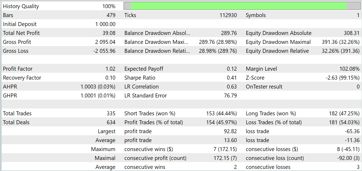
As you can see, the balance graph maintains a general upward trend. At the same time, 4 trends can be clearly identified on the chart: 2 profitable and 2 unprofitable. The positive thing is that profitable trends have more potential. This allows accumulating enough profit to avoid losing your deposit during a losing period. However, the balancing is very subtle. During the testing period, the profit factor was only 1.02, and the share of profitable trades was just below 46%.
Overall, the model shows potential, but more work is needed to minimize losing periods.
Conclusion
In this article, we discussed the FEDformer method, which was proposed for long-term time series forecasting. It includes an attention mechanism with low-rank frequency approximation and mixture decomposition to control the distribution shift.
In the practical part, we implemented our vision of the proposed approaches using MQL5. have trained and tested the model on real historical data. Testing results demonstrate the potential of the considered model. But at the same time, there are points that require additional attention.
References
- FEDformer: Frequency Enhanced Decomposed Transformer for Long-term Series Forecasting
- Other articles from this series
Programs used in the article
| # | Name | Type | Description |
|---|---|---|---|
| 1 | Research.mq5 | Expert Advisor | Example collection EA |
| 2 | ResearchRealORL.mq5 | Expert Advisor | EA for collecting examples using the Real-ORL method |
| 3 | Study.mq5 | Expert Advisor | Model training EA |
| 4 | StudyEncoder.mq5 | Expert Advisor | Encode Training EA |
| 5 | Test.mq5 | Expert Advisor | Model testing EA |
| 6 | Trajectory.mqh | Class library | System state description structure |
| 7 | NeuroNet.mqh | Class library | A library of classes for creating a neural network |
| 8 | NeuroNet.cl | Code Base | OpenCL program code library |
Translated from Russian by MetaQuotes Ltd.
Original article: https://www.mql5.com/ru/articles/14858
 How to integrate Smart Money Concepts (OB) coupled with Fibonacci indicator for Optimal Trade Entry
- Free trading apps
- Over 8,000 signals for copying
- Economic news for exploring financial markets
You agree to website policy and terms of use