Self Optimizing Expert Advisor with MQL5 And Python (Part III): Cracking The Boom 1000 Algorithm

MetaTrader 5 — Examples | 9 September 2024, 15:42

2 227

We will analyze all of Deriv’s synthetic markets individually, starting with their best known synthetic market, the Boom 1000. The Boom 1000 is notorious for its volatile and unpredictable behavior. The market is characterized by slow, short and equally sized bear candles that are randomly followed by violent, skyscraper sized bull candles. The bull candles are especially challenging to mitigate because the ticks associated with the candle normally aren’t sent to the client terminal, meaning that all stop losses are breached with guaranteed slippage every time.

Therefore, most successful traders have created strategies loosely based on only taking buy opportunities when trading the Boom 1000. Recall that the Boom 1000 could fall for 20 mins on the M1 chart, and retrace that entire movement in 1 candle! Therefore, given its overpowered bullish nature, successful traders look to use this to their advantage by attributing more weight to buy setups on the Boom 1000, than they would to a sell setup.

On the other hand, if we can simply create a new dependent variable, whose value depends on the price levels of Deriv’s synthetic instrument, we may have created a new relationship that we can model with more accuracy than we could capture when forecasting the Boom 1000. In other words, if we apply indicators to the market and model the indicator’s relationship with the market, we may obtain higher accuracy levels. Hopefully, our new target will not only render us higher accuracy levels, but furthermore it will be a faithful reflection of the actual changes in price. Meaning, if the indicator reading is expected to fall, price levels are also expected to fall. Recall that machine learning is centered around approximating a function assuming we have the inputs of that function, while we do not have any of the inputs that Deriv is using in their random number generator algorithm, by applying an indicator to their market, we have access to all the inputs the indicator depends on.

Methodology Overview

To assess the viability of the proposed strategy, we fetched 100000 rows of M1 data and the RSI indicator reading for each of those instances in time from our MetaTrader 5 terminal using a customized script I’ve written for us today. After reading in the script, we performed exploratory data analysis. We found that, 83% of the time when the RSI reading falls, price levels on the Boom 1000 also fall. This tells us that there is virtue in being able to predict the RSI value because it gives us an idea of where price levels will be. However, this also means that approximately 17% of the time the RSI will lead us astray.

We observed feeble correlation levels between the RSI and price levels on the Boom 1000, readings of 0.016. None of the scatter plots we performed exposed any discernible relationships in the data, we even attempted plotting in higher dimensions, but this too was in vain, the data appears quite challenging to separate effectively.

Our efforts did not stop there, we subsequently partitioned our data set into two halves, one half for training and optimizing and the second for validation and to test for overfitting. We also created two targets, one target captured the changes in price levels, whilst the second captured the changes in the RSI reading.

We proceeded to train two identical deep neural network classifiers to predict the changes in price levels and in the RSI levels respectively, the first model achieved accuracy levels of about 53% while the latter achieved accuracy levels of roughly 63%. Furthermore, the variance of our error levels when predicting the RSI changes was lower, implying that the latter model may have learned more effectively. Unfortunately, we were unable to tune our deep neural network without overfitting to the training set, this is suggested to us by the fact that we failed to outperform the default neural network on unseen validation data. We performed 5-fold time series cross-validation without random shuffling to measure our accuracy levels both in training and validation.

We selected the default RSI model as the best performing model and proceeded to export it to ONNX format and finally built our customized Boom 1000 AI-powered Expert Advisor in MQL5.

Fetching The Data

To get started, we first must fetch the data we need from our MetaTrader 5 terminal, this task is taken care of for us by our handy MQL5 script. The script I’ve written will fetch the market quotes associated with the Boom 1000, the timestamp of each candle and the relevant RSI reading before writing them out in CSV format for us. Notice that we set the RSI buffer as series before writing out the data, this step is crucial otherwise your RSI data will be in reverse chronological order, which is not what you want.

//+------------------------------------------------------------------+
//|                                                      ProjectName |
//|                                      Copyright 2020, CompanyName |
//|                                       http://www.companyname.net |
//+------------------------------------------------------------------+
#property copyright "Gamuchirai Zororo Ndawana"
#property link      "https://www.mql5.com/en/users/gamuchiraindawa"
#property version   "1.00"
#property script_show_inputs

//+------------------------------------------------------------------+
//| Script Inputs                                                    |
//+------------------------------------------------------------------+
input int size = 100000; //How much data should we fetch?

//+------------------------------------------------------------------+
//| Global variables                                                 |
//+------------------------------------------------------------------+
int rsi_handler;
double rsi_buffer[];


//+------------------------------------------------------------------+
//| On start function                                                |
//+------------------------------------------------------------------+
void OnStart()
  {

//--- Load indicator
   rsi_handler = iRSI(_Symbol,PERIOD_CURRENT,20,PRICE_CLOSE);
   CopyBuffer(rsi_handler,0,0,size,rsi_buffer);
   ArraySetAsSeries(rsi_buffer,true);

//--- File name
   string file_name = "Market Data " + Symbol() + ".csv";

//--- Write to file
   int file_handle=FileOpen(file_name,FILE_WRITE|FILE_ANSI|FILE_CSV,",");

   for(int i= size;i>=0;i--)
     {
      if(i == size)
        {
         FileWrite(file_handle,"Time","Open","High","Low","Close","RSI");
        }

      else
        {
         FileWrite(file_handle,iTime(Symbol(),PERIOD_CURRENT,i),
                   iOpen(Symbol(),PERIOD_CURRENT,i),
                   iHigh(Symbol(),PERIOD_CURRENT,i),
                   iLow(Symbol(),PERIOD_CURRENT,i),
                   iClose(Symbol(),PERIOD_CURRENT,i),
                   rsi_buffer[i]
                  );

         Print("Time: ",iTime(Symbol(),PERIOD_CURRENT,i),"Close: ",iClose(Symbol(),PERIOD_CURRENT,i),"RSI",rsi_buffer[i]);
        }
     }
//--- Close the file
   FileClose(file_handle);
  }
//+------------------------------------------------------------------+

Data Cleaning

We are now ready to start preparing our data for visualization. Let us first import the libraries we need.

#Import the libraries we need
import pandas as pd
import numpy as np

Display the library versions.

#Display library versions
print(f"Pandas version {pd.__version__}")
print(f"Numpy version {np.__version__}")

Pandas version 2.2.1
Numpy version 1.26.4

Now read in the CSV file.

#Read in the data we need
boom_1000 = pd.read_csv("Market Data Boom 1000 Index.csv")

Let’s see the data.

#Let's see the data
boom_1000

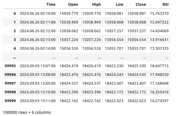
Fig 1: Our Boom 1000 market data

Let us now define our forecast horizon.

#Define how far into the future we should forecast
look_ahead = 20

We now need to define our forecast horizon, and also add additional labels to the data for visualization and plotting purposes.

#Let's add targets and labels for plotting
boom_1000["Price Target"] = boom_1000["Close"].shift(-look_ahead)
boom_1000["RSI Target"] = boom_1000["RSI"].shift(-look_ahead)

#Let's also add binary targets for plotting purposes
boom_1000["Price Binary Target"] = np.nan
boom_1000["RSI Binary Target"] = np.nan

#Label the binary targets
boom_1000.loc[boom_1000["Price Target"] < boom_1000["Close"],"Price Binary Target"] = 0
boom_1000.loc[boom_1000["Price Target"] > boom_1000["Close"],"Price Binary Target"] = 1

boom_1000.loc[boom_1000["RSI Target"] < boom_1000["RSI"],"RSI Binary Target"] = 0
boom_1000.loc[boom_1000["RSI Target"] > boom_1000["RSI"],"RSI Binary Target"] = 1

#Drop na values
boom_1000.dropna(inplace=True)

Let us now define our model inputs and the two targets we want to compare.

#Define the predictors and targets
predictors = ["Open","High","Low","Close","RSI"]
old_target = "Price Binary Target"
new_target = "RSI Binary Target"

Exploratory Data Analysis

Let us import the libraries we need.

#Exploratory data analysis
import seaborn as sns

Display the version of the library being used.

print(f"Seaborn version {sns.__version__}")
Seaborn version 0.13.2

Let us assess the purity of the signals generated by the RSI, purity in our sense answers this question “If the RSI level falls, will price levels fall too?” We calculated this quantity by first counting the number of instances whereby the RSI and Price Binary Target were not equal to each other, and then divided this count by the total number of rows in the entire data set, this quantity was subtracted from 1 to give us the total proportion of instances whereby the RSI and Price Binary Target were in harmony. According to our calculations, it appears that 83% of the time, the RSI and Price change in the same directions.

#Let's assess the purity of the signals generated
rsi_purity = 1 - boom_1000.loc[boom_1000["RSI Binary Target"] != boom_1000["Price Binary Target"]].shape[0] / boom_1000.shape[0]
print(f"Price and the RSI tend to move together {rsi_purity * 100}% of the time")

Price and the RSI tend to move together 83.69041189061593% of the time

This quantity is quite high, this gives us some levels of confidence that we may get good levels of separation when visualizing the data. Let us start off by creating a categorical plot to summarize all the instances where the RSI level fell, column 0, or rose, column 1 respectively on the x-axis, and the closing price is on the y-axis. We subsequently colored in each point, either blue or orange, to depict instances whereby the Boom 1000 price levels appreciated, or depreciated respectively. As we can see from the plot below, column 0 is mostly blue with a few patches of orange dots, and the opposite is true for column 1. This shows us that the RSI appears to be a good separator of price changes here. However, it is not perfect, we may need an additional indicator in the future.

#Let's see this purity level we just calculated
sns.catplot(data=boom_1000,x="RSI Binary Target",y="Close",hue="Price Binary Target")

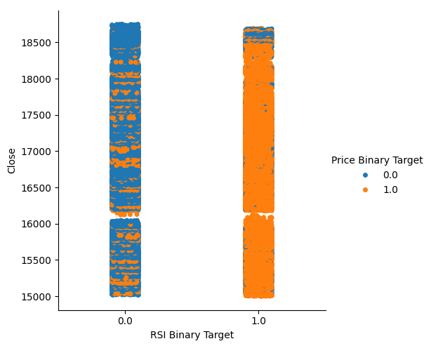
Fig 2: A categorical plot showing how well our RSI splits our data

We also created a scatter plot to try to visualize the relationship between the RSI and the Close price of the Boom 1000. Unfortunately, as we can see, there appears to be no relationship between the two. We observe long spaghetti like trails of haphazardly alternating blue and orange dots, this may indicate to us that there are other variables affecting the target.

#Let us also observe a scatter plot of the two
sns.scatterplot(data=boom_1000,x="RSI",y="Close",hue="Price Binary Target")

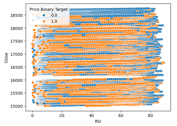
Fig 3:A scatter plot of our RSI readings against the close price

Perhaps the relationship we are trying to visualize can’t bee seen in two-dimensions, let us try visualizing the data in three-dimensions, hopefully we may observe the hidden interaction effects we are failing to see.

Import the libraries we need.

#Let's create 3D scatter plots
import matplotlib.pyplot as plt

Define how much data to plot.

#Define the plot end
end = 10000

Now create the 3D scatter plot. Unfortunately, we can still observe that the data appears randomly distributed with no observable patterns we can use to our advantage.

#Visualizing our data in 3D
fig = plt.figure(figsize=(7,7))
ax = fig.add_subplot(111,projection='3d')
colors = ['blue' if movement == 0 else 'red' for movement in boom_1000.loc[0:end,"Price Binary Target"]]
ax.scatter(boom_1000.loc[0:end,"RSI"],boom_1000.loc[0:end,"High"],boom_1000.loc[0:end,"Close"],c=colors)

ax.set_xlabel('Boom 1000 RSI')
ax.set_ylabel('Boom 1000 High')
ax.set_zlabel('Boom 1000 Close')

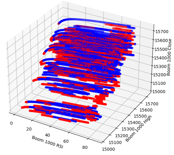
Fig 4: A 3D scatter plot of the Boom 1000 market and its relationship with the RSI

Let us now analyze the correlation levels between the RSI and our price data. We observe rather poor levels of correlation, almost 0 to be precise.

#Let's analyze the correlation levels
sns.heatmap(boom_1000.loc[:,predictors].corr(),annot=True)

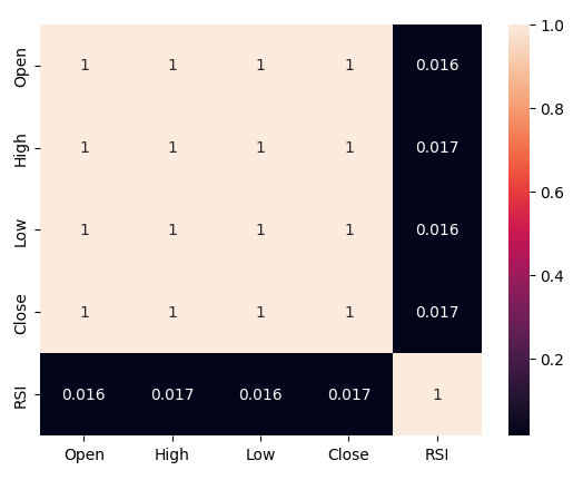
Fig 5: A heatmap of our correlation matrix

Preparing To Model The Data

Before we can start modeling our data, we first need to scale and standardize the data. First, let us import the libraries we need.

#Preparing to model the data
import sklearn
from sklearn.preprocessing import RobustScaler
from sklearn.neural_network import MLPClassifier,MLPRegressor
from sklearn.model_selection import TimeSeriesSplit, train_test_split
from sklearn.metrics import accuracy_score

Displaying the library version.

#Display library version
print(f"Sklearn version {sklearn.__version__}")

Sklearn version 1.4.1.post1

Scale the data.

#Scale our data
X = pd.DataFrame(RobustScaler().fit_transform(boom_1000.loc[:,predictors]),columns=predictors)

Defining our old and new targets.

#Our old and new target
old_y = boom_1000.loc[:,"Price Binary Target"]
new_y = boom_1000.loc[:,"RSI Binary Target"]

Performing the train test split.

#Perform train test splits
train_X,test_X,ohlc_train_y,ohlc_test_y = train_test_split(X,old_y,shuffle=False,test_size=0.5)
_,_,rsi_train_y,rsi_test_y = train_test_split(X,new_y,shuffle=False,test_size=0.5)

Prepare a data frame to store our accuracy levels in validation.

#Prepare data frames to store our accuracy levels
validation_accuracy = pd.DataFrame(index=np.arange(0,5),columns=["Close Accuracy","RSI Accuracy"])

Now let us create a time series spit object.

#Let's create the time series split object
tscv =  TimeSeriesSplit(gap=look_ahead,n_splits=5)

Modeling The Data

We are now ready to perform cross validation to observe the change in accuracy levels between the 2 possible targets.

#Instatiate the model
model = MLPClassifier(hidden_layer_sizes=(30,10),max_iter=200)
#Cross validate the model
for i,(train,test) in enumerate(tscv.split(train_X)):
        model.fit(train_X.loc[train[0]:train[-1],:],ohlc_train_y.loc[train[0]:train[-1]])
        validation_accuracy.iloc[i,0] = accuracy_score(ohlc_train_y.loc[test[0]:test[-1]],model.predict(train_X.loc[test[0]:test[-1],:]))

Our accuracy levels.

validation_accuracy

Close Accuracy	RSI Accuracy
0.53703	0.663186
0.544592	0.623575
0.479534	0.597647
0.57064	0.651422
0.545913	0.616373

Our mean accuracy levels instantly show us that we may be better off predicting changes in the RSI value.

validation_accuracy.mean()

Close Accuracy 0.535542
RSI Accuracy 0.630441
dtype: object

The lower the standard deviation, the more certainty the model has in its predictions. The model appears to have learned to forecast the RSI with more certainty than the changes in price.

validation_accuracy.std()

Close Accuracy 0.033765
RSI Accuracy 0.026613
dtype: object

Let us plot the performance of each of our models.

validation_accuracy.plot()

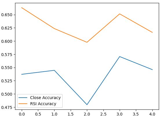
Fig 6: Visualizing our validation accuracy

Lastly, box plots help us observe the difference in performance between our two models. As we can see, the RSI model is outperforming the Price model by far.

#Our RSI validation accuracy is better
sns.boxplot(validation_accuracy)

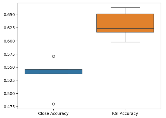
Fig 7: Box plots of our accuracy in validation

Feature Importance

Let us now analyze which features are important for predicting the RSI value, we will start off by performing forward selection on our Neural Network. Forward selection starts off with a null model and sequentially adds one feature at a time until no further enhancements can be made to the model’s performance.

First, we will import the libraries we need.

#Feature importance
import mlxtend
from mlxtend.feature_selection import SequentialFeatureSelector as SFS

Now display the library version.

print(f"Mlxtend version: {mlxtend.__version__}")

Mlxtend version: 0.23.1

Reinitialize the model.

#Reinitialize the model
model = MLPClassifier(hidden_layer_sizes=(30,10),max_iter=200)

Set up the feature selector.

#Define the forward feature selector
sfs1 = SFS(
        model,
        k_features=(1,X.shape[1]),
        n_jobs=-1,
        forward=True,
        cv=5,
        scoring="accuracy"
)

Fit the feature selector.

#Fit the feature selector
sfs = sfs1.fit(train_X,rsi_train_y)

Let us see the most important features we’ve identified. All the available features were selected.

sfs.k_feature_names_

('Open', 'High', 'Low', 'Close', 'RSI')

Let’s visualize the feature selection process. First, we import the libraries we need.

#Importing the libraries we need
from mlxtend.plotting import plot_sequential_feature_selection as plot_sfs
import matplotlib.pyplot as plt

Now we plot the results.

fig1 = plot_sfs(sfs.get_metric_dict(), kind='std_err')

plt.title('Sequential Forward Selection')
plt.grid()
plt.show()

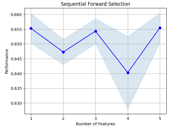
Fig 8: Visualizing the feature selection process

Mutual information (MI) allows us to gain an understanding of the potential each predictor has. The higher the MI score, generally the more useful the predictor may be. MI can capture non-linear dependencies in the data. Lastly, MI is on a logarithmic scale, meaning that MI scores above 3 are rare to see in practice.

Import the libraries we need.

#Let's analyze our MI scores
from sklearn.feature_selection import mutual_info_classif

Calculate MI scores.

mi_scores = pd.DataFrame(mutual_info_classif(train_X,rsi_train_y).reshape(1,5),columns=predictors)

Plotting the results shows us that the RSI column is the most important column according to MI.

#Let's visualize the results
mi_scores.plot.bar()

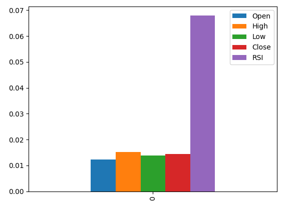
Fig 9: Visualizing our MI scores

Parameter Tuning

We will now attempt to tune our model to gain even more performance out of it. The RandomizedSearchCV module in the sklearn library allows us to easily tune our machine learning models. When tuning machine learning models, there is a tradeoff to be made between accuracy and compute time. We adjust the total number of iterations to decide between the two. Let us import the libraries we need.

#Parameter tuning
from sklearn.model_selection import RandomizedSearchCV

Initialize the model.

#Reinitialize the model
model = MLPClassifier(hidden_layer_sizes=(30,10),max_iter=200)

Define the tuner object.

#Define the tuner
tuner = RandomizedSearchCV(
        model,
        {
                "activation":["relu","tanh","logistic","identity"],
                "solver":["adam","sgd","lbfgs"],
                "alpha":[0.1,0.01,0.001,0.00001,0.000001],
                "learning_rate": ["constant","invscaling","adaptive"],
                "learning_rate_init":[0.1,0.01,0.001,0.0001,0.000001,0.0000001],
                "power_t":[0.1,0.5,0.9,0.01,0.001,0.0001],
                "shuffle":[True,False],
                "tol":[0.1,0.01,0.001,0.0001,0.00001],
        },
        n_iter=300,
        cv=5,
        n_jobs=-1,
        scoring="accuracy"
)

Fit the tuner object.

#Fit the tuner
tuner_results =tuner.fit(train_X,rsi_train_y)

The best parameters we’ve found.

#Best parameters
tuner_results.best_params_

{'tol': 1e-05,
'solver': 'lbfgs',
'shuffle': True,
'power_t': 0.0001,
'learning_rate_init': 0.01,
'learning_rate': 'adaptive',
'alpha': 1e-06,
'activation': 'logistic'}

Testing For Overfitting

To test for overfitting, we will cross-validate a default model and our customized model on the validation data. If our default model performs better, then we will know that we were overfitting the training set. Otherwise, we successfully performed hyperparameter tuning.

Initialize the 2 models.

#Testing for overfitting
default_model = MLPClassifier(hidden_layer_sizes=(30,10),max_iter=200)
customized_model = MLPClassifier(
                                hidden_layer_sizes=(30,10),
                                max_iter=200,
                                tol=0.00001,
                                solver="lbfgs",
                                shuffle=True,
                                power_t=0.0001,
                                learning_rate_init=0.01,
                                learning_rate="adaptive",
                                alpha=0.000001,
                                activation="logistic"
                                )

Fit both models on the training data.

#First we will train both models on the training set
default_model.fit(train_X,rsi_train_y)
customized_model.fit(train_X,rsi_train_y)

Reset the indexes on both data sets.

#Now we will reset our indexes
rsi_test_y = rsi_test_y.reset_index()
test_X = test_X.reset_index()

Format the data.

#Format the data
rsi_test_y = rsi_test_y.loc[:,"RSI Binary Target"]
test_X = test_X.loc[:,predictors]

Prepare a data frame to store our accuracy levels.

#Prepare a data frame to store our accuracy levels
validation_error = pd.DataFrame(index=np.arange(0,5),columns=["Default Neural Network","Customized Neural Network"])

Cross-validating each model to test for overfitting.

#Perform cross validation
for i,(train,test) in enumerate(tscv.split(test_X)):
        customized_model.fit(test_X.loc[train[0]:train[-1],predictors],rsi_test_y.loc[train[0]:train[-1]])
        validation_error.iloc[i,1] = accuracy_score(rsi_test_y.loc[test[0]:test[-1]],customized_model.predict(test_X.loc[test[0]:test[-1]]))

Our performance levels in validation.

validation_error

Default Neural Network	Customized Neural Network
0.627656	0.597767
0.637258	0.635938
0.621414	0.631977
0.6429	0.6411
0.664866	0.652503

Analyzing our mean performance levels clearly shows that the default model was slightly better than the customized model we have.

validation_error.mean()

Default Neural Network 0.638819
Customized Neural Network 0.631857
dtype: object

Furthermore, our customized model demonstrated more skill due to the lower variance in its accuracy scores.

validation_error.std()

Default Neural Network 0.016771
Customized Neural Network 0.020557
dtype: object

Let us plot our results.

validation_error.plot()

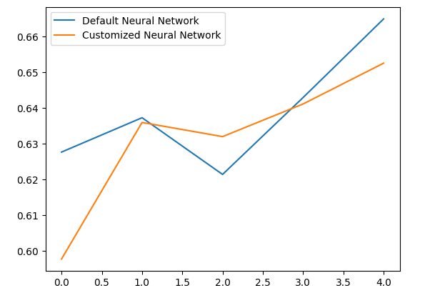
Fig 10: Visualizing our test for overfitting

The box plots show that our customized model appears less stable, it has outliers that we do not observe on the default model. Furthermore, our default model has slightly better average performance. Therefore, we will select the default model over the customized model.

sns.boxplot(validation_error)

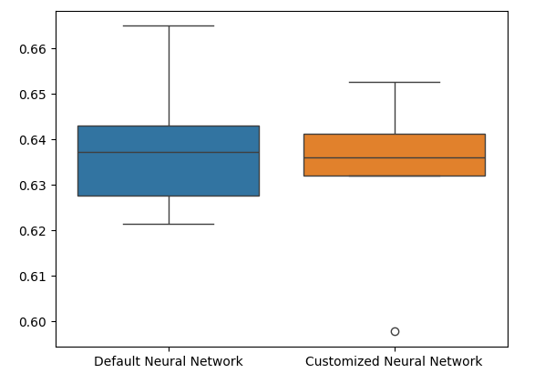
Fig 11: Visualizing our test for overfitting II

Preparing To Export To ONNX

Before we can export our model to ONNX format, we must first scale the data in a way we can reproduce in our MetaTrader 5 Terminal. We will subtract the column mean from each column and divide by the column standard deviation, this ensures that our model learn effectively since our data is on different scales. Also, we will export the mean and standard deviation values in CSV format so we can retrieve them later.

#Preparing to export to ONNX
#Let's scale our data
scaling_factors = pd.DataFrame(columns=predictors,index=['mean','standard deviation'])
X = boom_1000.loc[:,predictors]
y = boom_1000.loc[:,"RSI Target"]

Scale each column.

#Let's fill each column
for i in np.arange(0,len(predictors)):
        scaling_factors.iloc[0,i] = X.iloc[:,i].mean()
        scaling_factors.iloc[1,i] = X.iloc[:,i].std()
        X.iloc[:,i] = ( ( X.iloc[:,i] - scaling_factors.iloc[0,i] ) / scaling_factors.iloc[1,i])

Save the scaling factors in CSV format.

#Save the scaling factors as a CSV
scaling_factors.to_csv("/home/volatily/.wine/drive_c/Program Files/MetaTrader 5/MQL5/Files/boom_1000_scaling_factors.csv")

Exporting To ONNX

Open Neural Network Exchange (ONNX) is an open-source interoperable machine learning framework that allows developers to build, share and use machine learning models in any programming language that extends support to the ONNX API. This allows for us to build our machine learning models in Python and deploy them in MQL5 in production.

First, we will import the libraries we need.

#Exporting to ONNX
import onnx
import netron
import skl2onnx
from skl2onnx import convert_sklearn
from skl2onnx.common.data_types import FloatTensorType

Display the library versions.

#Display the library versions
print(f"Onnx version {onnx.__version__}")
print(f"Netron version {netron.__version__}")
print(f"Skl2onnx version {skl2onnx.__version__}")

Onnx version 1.15.0
Netron version 7.8.0
Skl2onnx version 1.16.0

Define our model’s input types.

#Define the model input types
initial_types = [("float_input",FloatTensorType([1,5]))]

Fit the model on all the data we have.

#Fit the model on all the data we have
default_model = MLPRegressor(hidden_layer_sizes=(30,10),max_iter=200)
default_model.fit(X,y)

Convert the model into its ONNX representation.

#Convert the model to an ONNX representation
onnx_model = convert_sklearn(default_model,initial_types=initial_types,target_opset=12)

Save the ONNX representation to file.

#Save the ONNX representation
onnx_name = "Boom 1000 Neural Network.onnx"
onnx.save(onnx_model,onnx_name)

View the model using netron.

#View the onnx model
netron.start(onnx_name)

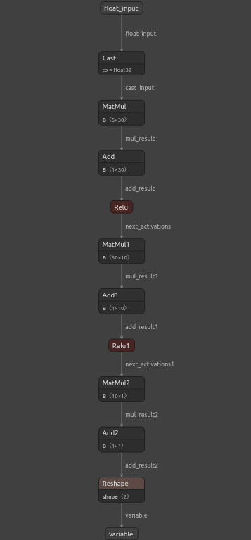
Fig 12: Visualizing our deep neural network

Visualizing our model's inputs and outputs

Fig 13: Visualizing our model's inputs and outputs

Implementation in MQL5

For us to build a trading application with an integrated AI-system, we will first require the ONNX model we just exported in Python.

//+------------------------------------------------------------------+
//|                                                    Boom 1000.mq5 |
//|                                        Gamuchirai Zororo Ndawana |
//|                          https://www.mql5.com/en/gamuchiraindawa |
//+------------------------------------------------------------------+
#property copyright "Gamuchirai Zororo Ndawana"
#property link      "https://www.mql5.com/en/gamuchiraindawa"
#property version   "1.00"

//+------------------------------------------------------------------+
//| ONNX Model                                                       |
//+------------------------------------------------------------------+
#resource "\\Files\\Boom 1000 Neural Network.onnx" as const uchar onnx_buffer[];

Let us also load the trade library for managing our positions.

//+-----------------------------------------------------------------+
//| Libraries we need                                               |
//+-----------------------------------------------------------------+
#include <Trade/Trade.mqh>
CTrade Trade;

Defining global variables that we will use throughout our program.

//+------------------------------------------------------------------+
//| Global variables                                                 |
//+------------------------------------------------------------------+
long onnx_model;
int rsi_handler,model_state,system_state;
double mean_values[5],std_values[5],rsi_buffer[],bid,ask;
vectorf model_outputs = vectorf::Zeros(1);
vectorf model_inputs = vectorf::Zeros(5);

Let us now define a function for preparing our ONNX model. This function will first create our model from the buffer we defined at the beginning of our program, and validate that the model is not corrupt, if it is corrupt, the function will return false and this will terminate the initialization procedure. From there, the function will proceed to set the input and output shapes of our ONNX model, if we fail to define either of the I/O parameters, our function will yet again return false and terminate the initialization procedure.

//+------------------------------------------------------------------+
//| This function will prepare our ONNX model                        |
//+------------------------------------------------------------------+
bool load_onnx_model(void)
  {
//--- First create the ONNX model from the buffer we created earlier
   onnx_model = OnnxCreateFromBuffer(onnx_buffer,ONNX_DEFAULT);

//--- Validate the ONNX model
   if(onnx_model == INVALID_HANDLE)
     {
      Comment("[ERROR] Failed to create the ONNX model: ",GetLastError());
      return(false);
     }

//--- Set the input and output shapes of the model
   ulong input_shape[] = {1,5};
   ulong output_shape[] = {1,1};

//--- Validate the input and output shape
   if(!OnnxSetInputShape(onnx_model,0,input_shape))
     {
      Comment("Failed to set the ONNX model input shape: ",GetLastError());
      return(false);
     }

   if(!OnnxSetOutputShape(onnx_model,0,output_shape))
     {
      Comment("Failed to set the ONNX model output shape: ",GetLastError());
      return(false);
     }

   return(true);
  }

We cannot use our ONNX model without scaling our model inputs, the following function will load the mean and standard deviation values we need into arrays we can easily access.

//+-----------------------------------------------------------------+
//| Load the scaling values                                         |
//+-----------------------------------------------------------------+
void load_scaling_values(void)
  {
//--- BOOM 1000 OHLC + RSI Mean values
   mean_values[0] = 16799.87389394667;
   mean_values[1] = 16800.872890865994;
   mean_values[2] = 16798.91007345616;
   mean_values[3] = 16799.908906749482;
   mean_values[4] = 43.45867626462568;
//--- BOOM 1000 OHLC + RSI Mean std values
   std_values[0] = 864.3356132780019;
   std_values[1] = 864.3839684000297;
   std_values[2] = 864.2859346216392;
   std_values[3] = 864.3344430387272;
   std_values[4] = 20.593175501388043;
  }
//+------------------------------------------------------------------+

We also need to define a function that will fetch updated market prices for us and our current technical indicator value.

//+------------------------------------------------------------------+
//| Fetch updated market prices and technical indicator values       |
//+------------------------------------------------------------------+
void update_market_data(void)
  {
//--- Market data
   bid = SymbolInfoDouble(Symbol(),SYMBOL_BID);
   ask = SymbolInfoDouble(Symbol(),SYMBOL_ASK);
//--- Technical indicator values
   CopyBuffer(rsi_handler,0,0,1,rsi_buffer);
  }

Finally, we need a function that will fetch our model’s inputs, scale them and fetch a prediction from our model. We will keep a flag to remember our model’s prediction, this will help us easily realize when our model is forecasting a reversal.

//+------------------------------------------------------------------+
//| Fetch a prediction from our model                                |
//+------------------------------------------------------------------+
void model_predict(void)
  {
//--- Get the model inputs
   model_inputs[0] = iOpen(_Symbol,PERIOD_CURRENT,0);
   model_inputs[1] = iHigh(_Symbol,PERIOD_CURRENT,0);
   model_inputs[2] = iLow(_Symbol,PERIOD_CURRENT,0);
   model_inputs[3] = iClose(_Symbol,PERIOD_CURRENT,0);
   model_inputs[4] = rsi_buffer[0];

//--- Scale the model inputs
   for(int i = 0; i < 5; i++)
     {
      model_inputs[i] = ((model_inputs[i] - mean_values[i]) / std_values[i]);
     }

//--- Fetch a prediction from our model
   OnnxRun(onnx_model,ONNX_DEFAULT,model_inputs,model_outputs);
//--- Give user feedback
   Comment("Model RSI Forecast: ",model_outputs[0]);
//--- Store the model's state
   if(rsi_buffer[0] > model_outputs[0])
     {
      model_state = -1;
     }

   else
      if(rsi_buffer[0] < model_outputs[0])
        {
         model_state = 1;
        }
  }

Now, we will define our model’s initialization procedure. We will start by loading our ONNX model, then fetching the scaling values and setting up or RSI indicator.

//+------------------------------------------------------------------+
//| Expert initialization function                                   |
//+------------------------------------------------------------------+
int OnInit()
  {
//--- This function will prepare our ONNX model and set the input and output shapes
   if(!load_onnx_model())
     {
      return(INIT_FAILED);
     }

//--- This function will prepare our scaling values
   load_scaling_values();

//--- Setup our technical indicatot
   rsi_handler = iRSI(Symbol(),PERIOD_CURRENT,20,PRICE_CLOSE);

//--- Everything went fine
   return(INIT_SUCCEEDED);
  }

Whenever our application has been removed from the chart, we will free up the resources we are no longer using, we will release the ONNX model, the RSI indicator and remove the Expert Advisor.

//+------------------------------------------------------------------+
//| Expert deinitialization function                                 |
//+------------------------------------------------------------------+
void OnDeinit(const int reason)
  {
//--- Release the resources we no longer need
   OnnxRelease(onnx_model);
   IndicatorRelease(rsi_handler);
   ExpertRemove();
  }

Whenever we receive updated prices, we will first fetch updated market and technical data, this includes the bid and ask prices as well as the RSI reading. Then we will be ready to fetch a new prediction from our model. If we have no open positions, we will follow our model’s prediction and remember our current position using a binary flag. Otherwise, if we have a position already open, we will check if our model’s new prediction is going against our open position, if it is, we will close our position. Otherwise, we will continue taking profits.

//+------------------------------------------------------------------+
//| Expert tick function                                             |
//+------------------------------------------------------------------+
void OnTick()
  {
//--- Fetch updated market prices
   update_market_data();

//--- On every tick we need to fetch a prediction from our model
   model_predict();

//--- If we have no open positions, follow the model's prediction
   if(PositionsTotal() == 0)
     {
      //--- Our model detected a spike
      if(model_state == 1)
        {
         Trade.Buy(0.2,Symbol(),ask,0,0,"BOOM 1000 AI");
         system_state = 1;
        }

      //--- Our model detected a drop
      if(model_state == -1)
        {
         Trade.Sell(0.2,Symbol(),bid,0,0,"BOOM 1000 AI");
         system_state = -1;
        }
     }

//--- If we have open positiosn, our AI system will decide when to close them
   else
      if(PositionsTotal() > 0)
        {
         if(system_state != model_state)
           {
            //--- Close the positions we opened
            Alert("Reversal detected by the AI system,closing all positions now!");
            Trade.PositionClose(Symbol());
           }
        }
  }
//+------------------------------------------------------------------+

Our system in action I

Fig 14: Our Boom 1000 system managed to catch a spike

Our system in action II

Fig 15: Our Boom 1000 system detected a reversal

Conclusion

In today's article we have demonstrated that it is possible to build self optimizing Expert Advisors to tackle even the most challenging of synthetic instruments, furthermore we have shown that the traditional approach of forecasting price levels directly would not suffice in today's algorithmic markets.

Attached files |

Download ZIP

Boom_1000_Neural_Network.onnx (2.8 KB)

Self_Optimizing_Expert_Advisors_in_Python_and_MQL5_4Part_IIIm.ipynb (1161.23 KB)

Fetch_One.mq5 (2.4 KB)

Boom_1000.mq5 (7.14 KB)

Warning: All rights to these materials are reserved by MetaQuotes Ltd. Copying or reprinting of these materials in whole or in part is prohibited.