
Reimagining Classic Strategies (Part VI): Multiple Time-Frame Analysis
Introduction
There are potentially infinite ways in which a modern investor can integrate Artificial Intelligence (AI) to enhance their trading decisions. Unfortunately, it is unlikely that you can evaluate all these strategies before deciding which strategy to trust with your hard-earned capital. In this series of articles, we will explore trading strategies to assess whether we can improve the strategy with AI. We aim to present you with the information you need to reach an informed decision whether this strategy is suitable for your individual investor profile.
Overview of Trading Strategy
In this article, we revisit a well-known strategy of multiple time-frame analysis. A large group of successful traders around the world hold the belief that there is virtue found in analyzing more than one time-frame before making investment decisions. There are many different variants of the strategy. However, they all tend to hold the general belief that whichever trend is identified on a higher time-frame, will persist on all time-frames lower than it.
So for example, if we observe bullish price behavior on the daily chart, then we would reasonably expect to see bullish price patterns on the hourly chart. This strategy also extends the idea further, according to the strategy, we should add more weight to price fluctuations that are aligned to the trend observed on the higher time-frame.
In other words, returning to our simple example, if we observed an uptrend on the daily chart, then we would be biased more towards buying opportunities on the hourly chart, and we would reluctantly take positions opposing the trend observed on the daily chart.
Generally speaking, the strategy falls apart when the trend observed on the higher time-frame is reversed. This is usually because the reversal will start out only on a lower time-frame. Recall that when using this strategy, little weight is attributed to fluctuations observed on lower time-frames that are contrary to the higher time-frame. Therefore, traders following this strategy would typically wait for the reversal to be observable on the higher time-frame. Therefore, they may experience a lot of volatility in price whilst waiting for confirmation from the higher time-frame.
Overview of Methodology
To assess the merits of this strategy empirically, we had to carefully extract meaningful data from our MetaTrader 5 Terminal. Our target in this article was predicting the future close price of the EURUSD 20 minutes into the future. To achieve this goal, we created 3 groups of predictors:
- Ordinary open, high, low and close price information.
- Changes in price levels across higher time-frames
- A superset of the above two sets.
We observed relatively weak levels of correlation between the ordinary price data and the changes in price on higher time-frames. The strongest correlation levels we observed were between the changes in price on the M15 and the price levels on the M1, approximately -0.1.
We created a large set of various models and trained them on all 3 sets of predictors to observe the changes in accuracy. Our best error levels were observed when using the first set of predictors, ordinary market data. From our observations, it appears that the linear regression model is the best performing model, followed by the Gradient Boosting Regressor (GBR) model.
Since the linear model does not have any tuning parameters of much interest to us, we selected the GBR model as our candidate solution, and the error levels of the linear model became our performance benchmark. Our goal now became to optimize the GBR model to surpass the benchmark performance set by the linear model.
Before we began the optimization process, we performed feature selection using the backward selection algorithm. All the features related to the changes in price across higher time-frames were discarded by the algorithm, possibly suggesting the relationship may not be reliable, or alternatively, we may also interpret this to suggest that we have not exposed the association to our model in a meaningful way.
We used a randomized search algorithm with 1000 iterations to find optimal settings for our GBR model. Afterward, we employed the results of our randomized search as the starting point for a local optimization of the continuous GBR parameters using the Limited Memory Broyden Fletcher Goldfarb And Shanno (L-BFGS-B) algorithm.
We failed to outperform the default GBR model on validation data, possibly indicating we were over-fitting to the training data. Furthermore, we also failed to surpass the linear model’s benchmark performance in validation.
Data Extraction
I’ve created a useful MQL5 scripts for extracting data from our MetaTrader 5 terminal. The script will also fetch the changes in price from a selection of higher time-frames and output the file in the path: “MetaTrader 5\MQL5\Files\...”
//+------------------------------------------------------------------+
//|                                                      ProjectName |
//|                                      Copyright 2020, CompanyName |
//|                                       http://www.companyname.net |
//+------------------------------------------------------------------+
#property copyright "Gamuchirai Zororo Ndawana"
#property link      "https://www.mql5.com/en/users/gamuchiraindawa"
#property version   "1.00"
#property script_show_inputs

//---Amount of data requested
input int size = 5; //How much data should we fetch?

//+------------------------------------------------------------------+
//|                                                                  |
//+------------------------------------------------------------------+
void OnStart()
  {
//---File name
   string file_name = "Market Data " + Symbol() + " multiple timeframe 20 step look ahead .csv";

//---Write to file
   int file_handle=FileOpen(file_name,FILE_WRITE|FILE_ANSI|FILE_CSV,",");

   for(int i= -1;i<=size;i++)
     {
      if(i == -1)
        {
         FileWrite(file_handle,"Time","Open","High","Low","Close","M5","M15","M30","H1","D1");
        }

      else
        {
         FileWrite(file_handle,iTime(Symbol(),PERIOD_CURRENT,i),
                   iOpen(Symbol(),PERIOD_CURRENT,i),
                   iHigh(Symbol(),PERIOD_CURRENT,i),
                   iLow(Symbol(),PERIOD_CURRENT,i),
                   iClose(Symbol(),PERIOD_CURRENT,i),
                   (iClose(Symbol(),PERIOD_M5,i) - iClose(Symbol(),PERIOD_M5,i+20)),
                   (iClose(Symbol(),PERIOD_M15,i) - iClose(Symbol(),PERIOD_M15,i+20)),
                   (iClose(Symbol(),PERIOD_M30,i) - iClose(Symbol(),PERIOD_M30,i+20)),
                   (iClose(Symbol(),PERIOD_H1,i) - iClose(Symbol(),PERIOD_H1,i+20)),
                   (iClose(Symbol(),PERIOD_D1,i) - iClose(Symbol(),PERIOD_D1,i+20))
                  );
        }
     }
//--- Close the file
FileClose(file_handle);
  }
//+------------------------------------------------------------------+
Reading in the Data
Let’s get started by loading the libraries we need.
import pandas as pd
imort numpy as np
Notice that the data is running from the near present, into the distant past. We need to reverse the data so that it runs from the past to the near present.
#Let's format the data so it starts with the oldest date
market_data = market_data[::-1]
market_data.reset_index(inplace=True)
Now we shall define our forecast horizon.
look_ahead = 20 Labeling the data. Our target will be the future close price of the EURUSD.
#Let's label the data
market_data["Target"] = market_data["Close"].shift(-look_ahead)
Now let us drop any rows with missing values.
#Drop rows with missing values
market_data.dropna(inplace=True)
Exploratory Data Analysis
Analyzing correlation levels.
#Let's see if there is any correlation
market_data.iloc[:,2:-1].corr()
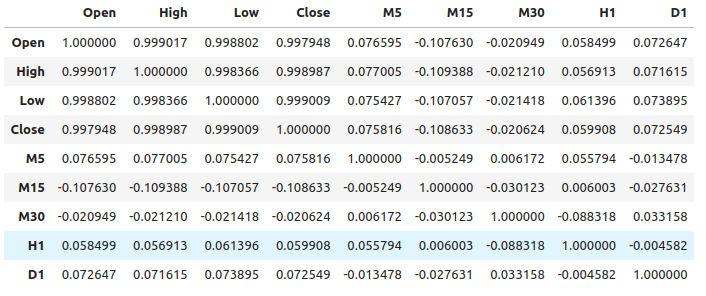
Fig 1: Correlation levels across different time-frames
As we can see, there are moderately weak levels of correlation in our dataset. Note, correlation does not necessarily prove there is a relationship between the variables being observed.
Mutual information is a measure of the potential a predictor has for explaining our target. Let us start off by considering a variable that we know definitely has strong potential for predicting the target, the open price.
from sklearn.feature_selection import mutual_info_regression
Now, as a benchmark, this is a good mutual information (MI) score.
#MI Score for the Open price
print(f'Open price has MI score: {mutual_info_regression(market_data.loc[:,["Open"]],market_data.loc[:,"Target"])[0]}') Let us now see the MI score for the changes in price on the M5 time-frame regarding the future price on the M1 time-frame.
#MI Score for the M5 change in price
print(f'M5 change in price has MI score: {mutual_info_regression(market_data.loc[:,["M5"]],market_data.loc[:,"Target"])[0]}') Our MI score in considerably smaller, this means we may not have exposed the relationship in a meaningful way, or maybe there is no dependency between the price levels on different time-frames!
#MI Score for the M15 change in price
print(f'M15 change in price has MI score: {mutual_info_regression(market_data.loc[:,["M15"]],market_data.loc[:,"Target"])[0]}') The same is true for the remaining time frames we selected.
Modelling the Relationship
Let us define our predictors and target.
#Let's define our predictors and our target
ohlc_predictors = [
        "Open",
        "High",
        "Low",
        "Close"
]

time_frame_predictors = [
        "M5",
        "M15",
        "M30",
        "H1",
        "D1"
]

all_predictors = ohlc_predictors + time_frame_predictors

target = "Target"
Now we import the libraries we need.
#Import the libraries we need
from sklearn.linear_model import LinearRegression
from sklearn.linear_model import SGDRegressor
from sklearn.ensemble import RandomForestRegressor
from sklearn.ensemble import BaggingRegressor
from sklearn.ensemble import GradientBoostingRegressor
from sklearn.ensemble import AdaBoostRegressor
from sklearn.neighbors import KNeighborsRegressor
from sklearn.svm import LinearSVR
from sklearn.neural_network import MLPRegressor
from sklearn.model_selection import TimeSeriesSplit,RandomizedSearchCV
from sklearn.metrics import root_mean_squared_error
from sklearn.preprocessing import RobustScaler
Define the parameters for our time-series split object.
#Define the time series split object
gap = look_ahead
splits = 10
Now let us prepare our models and also create data frames to store our accuracy levels. This way, we can observe the change in accuracy as we change our model inputs.
#Store our models in a list
models = [
        LinearRegression(),
        SGDRegressor(),
        RandomForestRegressor(),
        BaggingRegressor(),
        GradientBoostingRegressor(),
        AdaBoostRegressor(),
        KNeighborsRegressor(),
        LinearSVR(),
        MLPRegressor(hidden_layer_sizes=(10,4),early_stopping=True),
        MLPRegressor(hidden_layer_sizes=(100,20),early_stopping=True)
]

#Create a list of column titles for each model
columns = [
        "Linear Regression",
        "SGD Regressor",
        "Random Forest Regressor",
        "Bagging Regressor",
        "Gradient Boosting Regressor",
        "AdaBoost Regressor",
        "K Neighbors Regressor",
        "Linear SVR",
        "Small Neural Network",
        "Large Neurla Network"
]

#Create data frames to store our accuracy
ohlc_accuracy = pd.DataFrame(index=np.arange(0,10),columns=columns)
multiple_time_frame_accuracy = pd.DataFrame(index=np.arange(0,10),columns=columns)
all_accuracy = pd.DataFrame(index=np.arange(0,10),columns=columns)
Now let us prepare the predictors and scale our data.
#Preparing to perform cross validation
current_predictors = all_predictors
scaled_data = pd.DataFrame(RobustScaler().fit_transform(market_data.loc[:,all_predictors]),columns=all_predictors)
Create the time-series split object.
#Create the time series split object
tscv = TimeSeriesSplit(gap=gap,n_splits=splits)
Now we will perform cross-validation. The first loop iterates over the list of models we created earlier, the second loop cross-validates each model in turn.
#First we will iterate over all the available models
for i in np.arange(0,len(models)):
        #First select the model
        model = models[i]
        #Now we will cross validate this current model
        for j , (train,test) in enumerate(tscv.split(scaled_data)):
        #First define the train and test data
        train_X = scaled_data.loc[train[0]:train[-1],current_predictors]
        train_y = market_data.loc[train[0]:train[-1],target]
        test_X = scaled_data.loc[test[0]:test[-1],current_predictors]
        test_y = market_data.loc[test[0]:test[-1],target]
        #Now we will fit the model
        model.fit(train_X,train_y)
        #And finally record the accuracy
        all_accuracy.iloc[j,i] = root_mean_squared_error(test_y,model.predict(test_X))
Our accuracy levels when using ordinary inputs for our model.
ohlc_accuracy
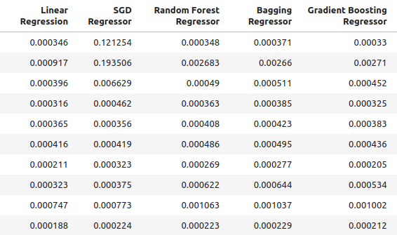
Fig 2: Our normal accuracy levels.
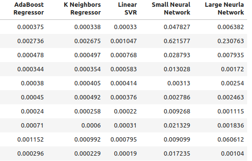
Fig 3: Our normal accuracy levels II
for i in np.arange(0,ohlc_accuracy.shape[1]):
    print(f"{columns[i]} had error levels {ohlc_accuracy.iloc[:,i].mean()}")
Linear Regression had error levels 0.00042256332959154886
SGD Regressor had error levels 0.0324320107406244
Random Forest Regressor had error levels 0.0006954883552094012
Bagging Regressor had error levels 0.0007030697054783931
Gradient Boosting Regressor had error levels 0.0006588749449742309
AdaBoost Regressor had error levels 0.0007159624774453208
K Neighbors Regressor had error levels 0.0006839218661791973
Linear SVR had error levels 0.000503277800807813
Small Neural Network had error levels 0.07740701832606754
Large Neural Network had error levels 0.03164056895135391
Our accuracy when using the new inputs we created.
multiple_time_frame_accuracy
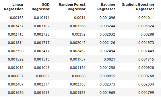
Fig 4: Our new accuracy levels
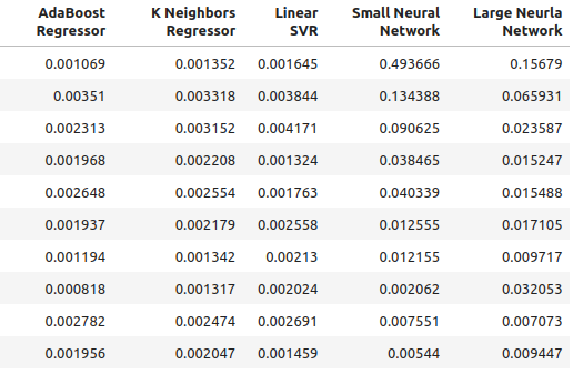
Fig 5: Our new accuracy levels II
for i in np.arange(0,ohlc_accuracy.shape[1]):
    print(f"{columns[i]} had error levels {multiple_time_frame_accuracy.iloc[:,i].mean()}")
Linear Regression had error levels 0.001913639795583766
SGD Regressor had error levels 0.0027638553835377206
Random Forest Regressor had error levels 0.0020041047670504254
Bagging Regressor had error levels 0.0020506512726394415
Gradient Boosting Regressor had error levels 0.0019180687958290775
AdaBoost Regressor had error levels 0.0020194136735787625
K Neighbors Regressor had error levels 0.0021943350208868213
Linear SVR had error levels 0.0023609474919917338
Small Neural Network had error levels 0.08372469596701271
Large Neural Network had error levels 0.035243897461061074
Lastly, let's observe our accuracy when using all available predictors.
all_accuracy
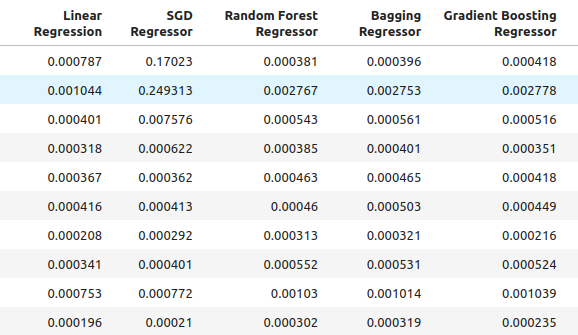
Fig 6: Our accuracy levels when using all the predictors we have.
for i in np.arange(0,ohlc_accuracy.shape[1]):
    print(f"{columns[i]} had error levels {all_accuracy.iloc[:,i].mean()}")
Linear Regression had error levels 0.00048307488099524497
SGD Regressor had error levels 0.043019079499194125
Random Forest Regressor had error levels 0.0007196920919204373
Bagging Regressor had error levels 0.0007263444909545053
Gradient Boosting Regressor had error levels 0.0006943964783049555
AdaBoost Regressor had error levels 0.0007217149661087063
K Neighbors Regressor had error levels 0.000872811528292862
Linear SVR had error levels 0.0006457525216512596
Small Neural Network had error levels 0.14002618062102
Large Neural Network had error levels 0.06774795252887988
As one can see, the linear model was the best performing model across all tests. Furthermore, it performed best when using ordinary OHLC data. However, the model does not have tuning parameters of interest to us. Therefore, we’ll select the second-best model, the Gradient Boosting Regressor (GBR), and attempt to outperform the linear model.
Feature Selection
Let us now see which features were most important to our GBR model.
#Feature selection
from mlxtend.feature_selection import SequentialFeatureSelector as SFS
Select the model.
#We'll select the Gradient Boosting Regressor as our chosen model
model = GradientBoostingRegressor()
We are going to use the backward selection algorithm. We will start off with a model that contains all predictors and continuously drop features one by one. A feature will only be dropped if it will result in improved performance from the model.
#Let us prepare the Feature Selector Object
sfs = SFS(model,
        k_features=(1,len(all_predictors)),
        forward=False,
        n_jobs=-1,
        scoring="neg_root_mean_squared_error",
        cv=10
        )
Performing feature selection.
#Select the best feature
sfs_results = sfs.fit(scaled_data.loc[:,all_predictors],market_data.loc[:,"Target"])
The algorithm only retained the high price and discarded all other features.
#The best feature we found
sfs_results.k_feature_names_
Let’s visualize our results.
#Prepare the plot
fig1 = plot_sfs(sfs_results.get_metric_dict(),kind="std_dev")
plt.title("Backward Selection on Gradient Boosting Regressor")
plt.grid()
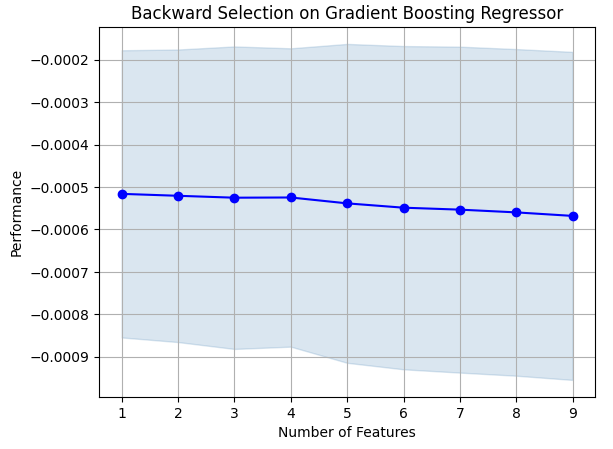
Fig 7: Visualizing the feature selection process
As one can see, as our model size and error levels were directly proportional. Or in other words, as our model got larger, so did our error levels.
Parameter Tuning
Let us now perform parameter tuning on our GBR model. We’ve identified 11 parameters from the model that are worth tuning, and we will allow 1000 iterations of the tuning object before we terminate the optimization process.
#Let us try to tune our model
from sklearn.model_selection import RandomizedSearchCV
Before we start tuning our model, let us partition our data into two. One half will be for training and optimizing our model, the latter will be used for validation and to test for over fitting.
#Before we try to tune our model, let's first create a train and test set
train_X = scaled_data.loc[:(scaled_data.shape[0]//2),:]
train_y = market_data.loc[:(market_data.shape[0]//2),"Target"]
test_X = scaled_data.loc[(scaled_data.shape[0]//2):,:]
test_y = market_data.loc[(market_data.shape[0]//2):,"Target"]
Define the tuning object.
#Time the process
import time

start_time = time.time()

#Prepare the tuning object
tuner = RandomizedSearchCV(GradientBoostingRegressor(),
                        {
                                "loss": ["squared_error","absolute_error","huber"],
                                "learning_rate": [0,(10.0 ** -1),(10.0 ** -2),(10.0 ** -3),(10.0 ** -4),(10.0 ** -5),(10.0 ** -6),(10.0 ** -7)],
                                "n_estimators": [5,10,25,50,100,200,500,1000],
                                "max_depth": [1,2,3,5,9,10],
                                "min_samples_split":[0.1,0.2,0.3,0.4,0.5,0.6,0.7,0.8,0.9,1.0],
                                "criterion":["friedman_mse","squared_error"],
                                "min_samples_leaf":[0.1,0.2,0.3,0.4,0.5,0.6,0.7,0.8,0.9],
                                "min_weight_fraction_leaf":[0.0,0.1,0.2,0.3,0.4,0.5],
                                "max_features":[1,2,3,4,5,20],
                                "max_leaf_nodes": [2,3,4,5,10,20,50,90,None],
                                "min_impurity_decrease": [0,1,10,(10.0 ** 2),(10.0 ** 3),(10.0 ** 4)]
                        },
                        cv=5,
                        n_iter=1000,
                        return_train_score=False,
                        scoring="neg_mean_squared_error"
                        )
Tune the GBR model.
#Tune the GradientBoostingRegressor
tuner.fit(train_X,train_y)

end_time = time.time()

print(f"Process completed in {end_time - start_time} seconds.")
Let’s see the results in order of best to worst.
#Let's observe the results
tuner_results = pd.DataFrame(tuner.cv_results_)
params = ["param_loss",
          "param_learning_rate",
          "param_n_estimators",
          "param_max_depth",
          "param_min_samples_split",
          "param_criterion",
          "param_min_samples_leaf",
          "param_max_features",
          "param_max_leaf_nodes",
          "param_min_impurity_decrease",
          "param_min_weight_fraction_leaf",
          "mean_test_score"]
tuner_results.loc[:,params].sort_values(by="mean_test_score",ascending=False)
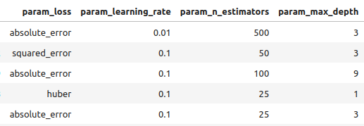
Fig 8: Some of our best results.

Fig 9: Some of our best results II

Fig 10: Some of our best results III
The best parameters we found.
#Best parameters we found
tuner.best_params
{'n_estimators': 500,
'min_weight_fraction_leaf': 0.0,
'min_samples_split': 0.4,
'min_samples_leaf': 0.1,
'min_impurity_decrease': 1,
'max_leaf_nodes': 10,
'max_features': 2,
'max_depth': 3,
'loss': 'absolute_error',
'learning_rate': 0.01,
'criterion': 'friedman_mse'}
Deeper Parameter Tuning

Fig 11: The SciPy logo
SciPy is a Python library used for scientific computation. SciPy stands for scientific python. Let us see if we can’t find even better parameters. We will use the SciPy optimize library to try to find parameters that will improve our model’s performance.
#Let's see if we can't find better parameters
#We may be overfitting the training data!
from scipy.optimize import minimize
To use the SciPy optimize library, we need to define an objective function. Our objective function will the average of the cross validated error levels our model achieves on the training set. Our SciPy optimizer will search for coefficients that reduce our training error.
#Define the objective function
def objective(x):
        #Create a dataframe to store our new accuracy
        current_error = pd.DataFrame(index=[0],columns=["error"])
        #x is an array of possible values to use for our Gradient Boosting Regressor
        model = GradientBoostingRegressor(n_estimators=500,
                                        min_impurity_decrease=1,
                                        max_leaf_nodes=10,
                                        max_features=2,
                                        max_depth=3,
                                        loss="absolute_error",
                                        criterion="friedman_mse",
                                        min_weight_fraction_leaf=x[0],
                                        min_samples_split=x[1],
                                        min_samples_leaf=x[2],
                                        learning_rate=x[3])
        model.fit(train_X.loc[:,:],train_y.loc[:])
        current_error.iloc[0,0] = root_mean_squared_error(train_y.loc[:],model.predict(train_X.loc[:,:]))
        #Record our progress
        mean_error = current_error.loc[:].mean()
        #Return the average error
        return mean_error
Now let us begin the optimization process. Note, some parameters in the GBR model do not allow negative values and our SciPy optimizer will pass negative values unless we specify bounds for the optimizer. Furthermore, the optimizer expects us to give it a starting point. We will use the endpoint of the previous optimization algorithm as the starting point for this one.
#Let's optimize these parameters again
#Fist define the bounds
bounds = ((0.0,0.5),(0.3,0.5),(0.001,0.2),(0.001,0.1))

#Then define the starting points for the L-BFGS-B algorithm
pt = np.array([tuner.best_params_["min_weight_fraction_leaf"],
                tuner.best_params_["min_samples_split"],
                tuner.best_params_["min_samples_leaf"],
                tuner.best_params_["learning_rate"]
                ])
Minimizing training error.
lbfgs = minimize(objective,pt,bounds=bounds,method="L-BFGS-B")
Let’s see the results.
lbfgs
success: True
status: 0
fun: 0.0005766670348377334
x: [ 5.586e-06 4.000e-01 1.000e-01 1.000e-02]
nit: 3
jac: [-6.216e+00 -4.871e+02 -2.479e+02 8.882e+01]
nfev: 180
njev: 36
hess_inv: <4x4 LbfgsInvHessProduct with dtype=float64>
Testing For Over-fitting
Let us now compare the accuracy of our 2 customized models against the default GBR model. Furthermore, we will also pay attention to see if we outperformed the linear model.
#Let us now see how well we're performing on the validation set
linear_regression = LinearRegression()
default_gbr = GradientBoostingRegressor()
grid_search_gbr = GradientBoostingRegressor(n_estimators=500,
                                        min_impurity_decrease=1,
                                        max_leaf_nodes=10,
                                        max_features=2,
                                        max_depth=3,
                                        loss="absolute_error",
                                        criterion="friedman_mse",
                                        min_weight_fraction_leaf=0,
                                        min_samples_split=0.4,
                                        min_samples_leaf=0.1,
                                        learning_rate=0.01
                                        )
lbfgs_grid_search_gbr = GradientBoostingRegressor(
                                        n_estimators=500,
                                        min_impurity_decrease=1,
                                        max_leaf_nodes=10,
                                        max_features=2,
                                        max_depth=3,
                                        loss="absolute_error",
                                        criterion="friedman_mse",
                                        min_weight_fraction_leaf=lbfgs.x[0],
                                        min_samples_split=lbfgs.x[1],
                                        min_samples_leaf=lbfgs.x[2],
                                        learning_rate=lbfgs.x[3]
                                        )
Our accuracy with the linear model.
#Linear Regression
linear_regression.fit(train_X,train_y)
root_mean_squared_error(test_y,linear_regression.predict(test_X)) Our accuracy with the default GBR model.
#Default Gradient Boosting Regressor
default_gbr.fit(train_X,train_y)
root_mean_squared_error(test_y,default_gbr.predict(test_X)) Our accuracy with the GBR model customized by random search.
#Random Search Gradient Boosting Regressor
grid_search_gbr.fit(train_X,train_y)
root_mean_squared_error(test_y,grid_search_gbr.predict(test_X)) Our accuracy when using the GBR model customized by random search and L-BFGS-B.
#L-BFGS-B Random Search Gradient Boosting Regressor
lbfgs_grid_search_gbr.fit(train_X,train_y)
root_mean_squared_error(test_y,lbfgs_grid_search_gbr.predict(test_X))
As we can see, we failed to outperform the linear model. Also, we failed to outperform the default GBR model. Therefore, we will progress onward with the default GBR model for the sake of demonstration. However, note that selecting the linear model would’ve given us more accuracy.
Exporting to ONNX
Open Neural Network Exchange (ONNX) is a protocol that allows us to represent machine learning models as a computational graph of nodes and edges. Where nodes represent mathematical operations and edges represent the flow of data. By exporting our machine learning model to ONNX format, we will be able to use our AI models inside our Expert Advisor with ease.
Let us get ready to export our ONNX model.
#We failed to beat the linear regression model, in such cases we should pick the linear model!
#However for demonstrational purposes we'll pick the gradient boosting regressor
#Let's export the default GBR to ONNX format
from skl2onnx.common.data_types import FloatTensorType
from skl2onnx import convert_sklearn
import onnx
Now we need to scale our data in a way that we can reproduce in MetaTrader 5. The easiest transformation is simply subtracting the mean, and dividing by the standard deviation.
#We need to save the scale factors for our inputs
scale_factors = pd.DataFrame(index=["mean","standard deviation"],columns=all_predictors)

for i in np.arange(0,len(all_predictors)):
        scale_factors.iloc[0,i] = market_data.iloc[:,i+2].mean()
        scale_factors.iloc[1,i] = market_data.iloc[:,i+2].std()
        market_data.iloc[:,i+2] = ((market_data.iloc[:,i+2] - market_data.iloc[:,i+2].mean()) / market_data.iloc[:,i+2].std())

scale_factors

Fig 12: Our scale factors
Define the input types for our ONNX model.
#Define our initial types
initial_types = [("float_input",FloatTensorType([1,test_X.shape[1]]))]
Fitting the model on all the data we have.
#Fit the model on all the data we have
model = GradientBoostingRegressor().fit(market_data.loc[:,all_predictors],market_data.loc[:,"Target"])
Create the ONNX representation.
#Create the ONNX representation
onnx_model = convert_sklearn(model,initial_types=initial_types,target_opset=12)
Save the ONNX model.
#Now save the ONNX model
onnx_model_name = "GBR_M1_MultipleTF_Float.onnx"
onnx.save(onnx_model,onnx_model_name)
Visualizing the Model
Netron is an open-source visualizer for inspecting machine learning models. Currently, netron offers support for a limited number of frameworks. However, as time progresses and as the library matures, support will be extended to different machine learning frameworks.
Import the libraries we need.
#Import netron so we can visualize the model
import netron
Launch netron.
netron.start(onnx_model_name)
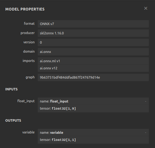
Fig 13: Our Gradient Boosting Regressor ONNX model properties
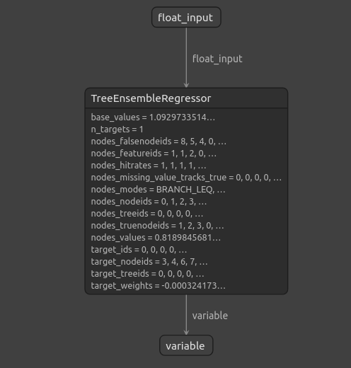 \
\
Fig 14: The structure of our Gradient Boosting Regressor
As we can see the input and output shape of our ONNX model are where we expect them to be, this gives us confidence to proceed and build an Expert Advisor on top of our ONNX model.
Implementing in MQL5
To start building our Expert Advisor with an integrated AI module, we first need to require the ONNX model.//+------------------------------------------------------------------+ //| Multiple Time Frame.mq5 | //| Gamuchirai Zororo Ndawana | //| https://www.mql5.com/en/gamuchiraindawa | //+------------------------------------------------------------------+ #property copyright "Gamuchirai Zororo Ndawana" #property link "https://www.mql5.com/en/gamuchiraindawa" #property version "1.00" //+------------------------------------------------------------------+ //| Require the onnx file | //+------------------------------------------------------------------+ #resource "\\Files\\GBR_M1_MultipleTF_Float.onnx" as const uchar onnx_model_buffer[];
Now we will load the trade library.
//+------------------------------------------------------------------+
//| Libraries we need                                                |
//+------------------------------------------------------------------+
#include <Trade/Trade.mqh>
CTrade Trade;
Let us define inputs our end user can change.
//+------------------------------------------------------------------+
//| Inputs                                                           |
//+------------------------------------------------------------------+
input double max_risk = 20;               //How much profit/loss should we allow before closing
input double sl_width = 1;                //How wide should out sl be?
Now we shall define global variables that will be used throughout our program.
//+------------------------------------------------------------------+
//| Global variables                                                 |
//+------------------------------------------------------------------+
long onnx_model;                          //Our onnx model
double mean_variance[9],std_variance[9];  //Our scaling factors
vector model_forecast = vector::Zeros(1); //Model forecast
vector model_inputs = vector::Zeros(9);   //Model inputs
double ask,bid;                           //Market prices
double trading_volume;                    //Our trading volume
int lot_multiple = 20;                    //Our lot size
int state = 0;                            //System state
Let us define helper functions that we will use throughout our program. First, we need a function to detect reversals and alert the end user about the danger ahead that our AI system has predicted. If our AI system detects a reversal, we will close the open positions we have in that market.
//+------------------------------------------------------------------+
//| Check reversal                                                   |
//+------------------------------------------------------------------+
void check_reversal(void)
  {
//--- Check for reversal
   if(((state == 1) && (model_forecast[0] < iClose(Symbol(),PERIOD_M1,0))) || ((state == 2) && (model_forecast[0] > iClose(Symbol(),PERIOD_M1,0))))
     {
      Alert("Reversal predicted.");
      Trade.PositionClose(Symbol());
     }
//--- Check if we have breached our maximum risk levels
   if(MathAbs(PositionGetDouble(POSITION_PROFIT) > max_risk))
     {
      Alert("We've breached our maximum risk level.");
      Trade.PositionClose(Symbol());
     }
  }
Now we will define a function to find market entry opportunities. We will only consider an entry to be valid if we have confirmation from higher time-frames regarding the move. In this Expert Advisor, we want our trades to align with price action on the weekly chart.
//+------------------------------------------------------------------+
//| Find an entry                                                    |
//+------------------------------------------------------------------+
void find_entry(void)
  {
//--- Analyse price action on the weekly time frame
   if(iClose(Symbol(),PERIOD_W1,0) > iClose(Symbol(),PERIOD_W1,20))
     {
      //--- We are riding bullish momentum
      if(model_forecast[0] > iClose(Symbol(),PERIOD_M1,20))
        {
         //--- Enter a buy
         Trade.Buy(trading_volume,Symbol(),ask,(ask - sl_width),(ask + sl_width),"Multiple Time Frames AI");
         state = 1;
        }
     }
//--- Analyse price action on the weekly time frame
   if(iClose(Symbol(),PERIOD_W1,0) < iClose(Symbol(),PERIOD_W1,20))
     {
      //--- We are riding bearish momentum
      if(model_forecast[0] < iClose(Symbol(),PERIOD_M1,20))
        {
         //--- Enter a sell
         Trade.Sell(trading_volume,Symbol(),bid,(bid + sl_width),(bid - sl_width),"Multiple Time Frames AI");
         state = 2;
        }
     }
  }
We also need a function to fetch current market prices.
//+------------------------------------------------------------------+
//| Update market prices                                             |
//+------------------------------------------------------------------+
void update_market_prices(void)
  {
   ask = SymbolInfoDouble(Symbol(),SYMBOL_ASK);
   bid = SymbolInfoDouble(Symbol(),SYMBOL_BID);
  }
Our ONNX model cannot be used unless we standardize and normalize the inputs, this function will fetch the scaling factors we used when training our ONNX model.
//+------------------------------------------------------------------+
//| Load our scaling factors                                         |
//+------------------------------------------------------------------+
void load_scaling_factors(void)
  {
//--- EURUSD OHLC
   mean_variance[0] = 1.0930010861272836;
   std_variance[0] = 0.0017987600829890852;
   mean_variance[1] = 1.0930721822927123;
   std_variance[1] =  0.001810556238082839;
   mean_variance[2] = 1.092928371812889;
   std_variance[2] = 0.001785041172362313;
   mean_variance[3] = 1.093000590242923;
   std_variance[3] = 0.0017979420556511476;
//--- M5 Change
   mean_variance[4] = (MathPow(10.0,-5) * 1.4886568962056413);
   std_variance[4] = 0.000994902152654042;
//--- M15 Change
   mean_variance[5] = (MathPow(10.0,-5) * 1.972093957036524);
   std_variance[5] = 0.0017104874192072138;
//--- M30 Change
   mean_variance[6] = (MathPow(10.0,-5) * 1.5089339490060967);
   std_variance[6] = 0.002436078407827825;
//--- H1 Change
   mean_variance[7] = 0.0001529512146155358;
   std_variance[7] = 0.0037675774501395387;
//--- D1 Change
   mean_variance[8] = -0.0008775667536639223;
   std_variance[8] = 0.03172437243836734;
  }
Defining the function responsible for fetching predictions from our model, note that we are scaling the inputs before passing them to our ONNX model. Predictions are obtained from the model using the OnnxRun command.
//+------------------------------------------------------------------+
//| Model predict                                                    |
//+------------------------------------------------------------------+
void model_predict(void)
  {
//--- EURD OHLC
   model_inputs[0] = ((iClose(Symbol(),PERIOD_CURRENT,0) - mean_variance[0]) / std_variance[0]);
   model_inputs[1] = ((iClose(Symbol(),PERIOD_CURRENT,0) - mean_variance[1]) / std_variance[1]);
   model_inputs[2] = ((iClose(Symbol(),PERIOD_CURRENT,0) - mean_variance[2]) / std_variance[2]);
   model_inputs[3] = ((iClose(Symbol(),PERIOD_CURRENT,0) - mean_variance[3]) / std_variance[3]);
//--- M5 CAHNGE
   model_inputs[4] = (((iClose(Symbol(),PERIOD_M5,0) - iClose(Symbol(),PERIOD_M5,20)) - mean_variance[4]) / std_variance[4]);
//--- M15 CHANGE
   model_inputs[5] = (((iClose(Symbol(),PERIOD_M15,0) - iClose(Symbol(),PERIOD_M15,20)) - mean_variance[5]) / std_variance[5]);
//--- M30 CHANGE
   model_inputs[6] = (((iClose(Symbol(),PERIOD_M30,0) - iClose(Symbol(),PERIOD_M30,20)) - mean_variance[6]) / std_variance[6]);
//--- H1 CHANGE
   model_inputs[7] = (((iClose(Symbol(),PERIOD_H1,0) - iClose(Symbol(),PERIOD_H1,20)) - mean_variance[7]) / std_variance[7]);
//--- D1 CHANGE
   model_inputs[8] = (((iClose(Symbol(),PERIOD_D1,0) - iClose(Symbol(),PERIOD_D1,20)) - mean_variance[8]) / std_variance[8]);
//--- Fetch forecast
   OnnxRun(onnx_model,ONNX_DEFAULT,model_inputs,model_forecast);
  }
Now we will define a function to load our Onnx model and define the input and output shape.
//+------------------------------------------------------------------+
//| Load our onnx file                                               |
//+------------------------------------------------------------------+
bool load_onnx_file(void)
  {
//--- Create the model from the buffer
   onnx_model = OnnxCreateFromBuffer(onnx_model_buffer,ONNX_DEFAULT);

//--- Set the input shape
   ulong input_shape [] = {1,9};

//--- Check if the input shape is valid
   if(!OnnxSetInputShape(onnx_model,0,input_shape))
     {
      Alert("Incorrect input shape, model has input shape ", OnnxGetInputCount(onnx_model));
      return(false);
     }

//--- Set the output shape
   ulong output_shape [] = {1,1};

//--- Check if the output shape is valid
   if(!OnnxSetOutputShape(onnx_model,0,output_shape))
     {
      Alert("Incorrect output shape, model has output shape ", OnnxGetOutputCount(onnx_model));
      return(false);
     }
//--- Everything went fine
   return(true);
  }
//+------------------------------------------------------------------+
We can now define the program’s initialization procedure. Our Expert will load the Onnx file, load the scaling factors and fetch market data.
//+------------------------------------------------------------------+
//| Expert initialization function                                   |
//+------------------------------------------------------------------+
int OnInit()
  {
//--- Load the ONNX file
   if(!load_onnx_file())
     {
      //--- We failed to load our onnx model
      return(INIT_FAILED);
     }

//--- Load scaling factors
   load_scaling_factors();

//--- Get trading volume
   trading_volume = SymbolInfoDouble(Symbol(),SYMBOL_VOLUME_MIN) * lot_multiple;

//--- Everything went fine
   return(INIT_SUCCEEDED);
  }
Whenever our program is not in use, we will free up the resources we no longer need. We will release the Onnx model and remove the expert advisor from the chart.
//+------------------------------------------------------------------+
//| Expert deinitialization function                                 |
//+------------------------------------------------------------------+
void OnDeinit(const int reason)
  {
//--- Release the resources we used for our onnx model
   OnnxRelease(onnx_model);

//--- Release the expert advisor
   ExpertRemove();
  }
Whenever we have new prices being offered, we will first fetch a prediction from our model and then update our market prices. If we have no open position, we will try to find an entry. Otherwise, if we have a position that needs to be managed, we will attentively be on the look-out for a possible reversal.
//+------------------------------------------------------------------+
//| Expert tick function                                             |
//+------------------------------------------------------------------+
void OnTick()
  {
//--- We always need a prediction from our model
   model_predict();

//--- Show the model forecast
   Comment("Model forecast ",model_forecast);

//--- Fetch market prices
   update_market_prices();

//--- If we have no open positions, find an entry
   if(PositionsTotal() == 0)
     {
      //--- Find entry
      find_entry();
      //--- Update state
      state = 0;
     }

//--- If we have an open position, manage it
   else
     {
      //--- Check if our AI is predicting a reversal
      check_reversal();
     }
  }
Now we can see our application in action.
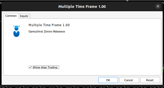
Fig 15: Our Expert Advisor Interface
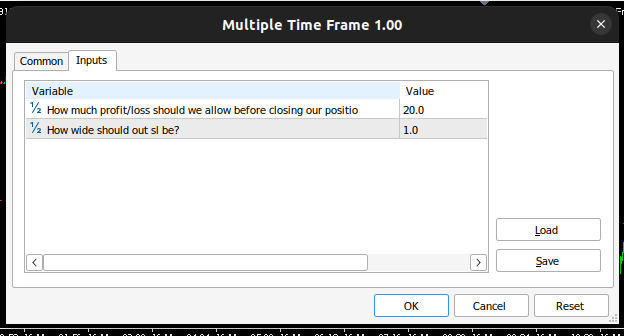
Fig 16: Our Expert Advisor Inputs
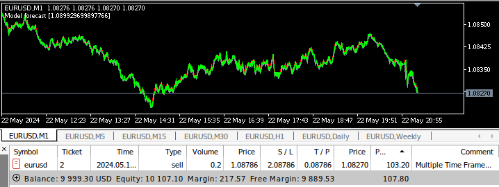
Fig 17: Multiple Time-Frame Expert Advisor being back tested
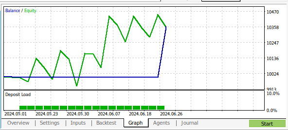
Fig 18:The results of back testing our program over 1 month of M1 data
Conclusion
In this article, we have demonstrated that it is possible to build an AI-powered Expert Advisor that analyzes multiple time frames. Although we obtained higher accuracy levels using ordinary OHLC data, there are many different choices we didn't examine, for example we didn't add any indicators on higher time-frames. There are many ways we can apply AI into our trading strategy, hopefully you now have new ideas of the capabilities waiting to be tapped in your installation of MetaTrader 5.
Warning: All rights to these materials are reserved by MetaQuotes Ltd. Copying or reprinting of these materials in whole or in part is prohibited.
This article was written by a user of the site and reflects their personal views. MetaQuotes Ltd is not responsible for the accuracy of the information presented, nor for any consequences resulting from the use of the solutions, strategies or recommendations described.
 Developing a multi-currency Expert Advisor (Part 7): Selecting a group based on forward period
 Integrating MQL5 with data processing packages (Part 2): Machine Learning and Predictive Analytics
 Creating a Trading Administrator Panel in MQL5 (Part I): Building a Messaging Interface
 Non-stationary processes and spurious regression
- Free trading apps
- Over 8,000 signals for copying
- Economic news for exploring financial markets
You agree to website policy and terms of use
Thank you for your step by step and detailed analysis. This is really helpfully as a template for those unfamiliar with data analysis to work through . the result is fascinating (and unexpected), Does this mean we should be testing other parameters as well e.g. volume, spread Previous day action or is that more overfitting. Thanks for the template I now have the tools to check it myself :)