Matrix Factorization: The Basics

Introduction

Welcome everyone to my new article with educational content.

In this article, we will talk about matrix calculations. Dear readers, do not rush to refuse reading this article, thinking that we will talk about something purely mathematical and too complicated. Contrary to what many people think, a good programmer is not someone who writes a giant program that only they can understand, or someone who writes code in a trendy programming language. A real and good programmer understands that a computer is nothing more than a computing machine to which we can tell how computations should be performed. It doesn't matter what exactly we are creating, it can be a simple text editor that does not contain any mathematical code. But this is just an illusion. Even a text editor contains a fair amount of math in its code, especially if it has a spell checker built into it.

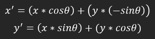
Basically, in programming, there are two ways to perform factorization or calculations if you prefer to call them that. The first way is to calculate in scalar form, that is, by using the functions provided by the language, to write the formula as shown below:

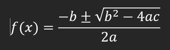
This formula that anyone can recognize allows you to calculate the roots of a quadratic function. It can be easily written in any programming language using the functions and resources available in that language. But there is another way of to make calculations.: matrix or vector, as some people prefer to call it. In this article, we will call it "matrix" because we will use matrices to represent things. This type of factoring looks like this:

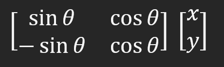
Some enthusiasts who are just starting out in programming have no idea how to write this in code. They end up converting matrix notation to scalar notation to get the same result.

The question is not whether it is right or wrong. If the result obtained is correct, then it does not matter much. In this case, this matrix shows that something rotates around a given point. In this article, I want to show you, dear readers, how you can, using MQL5 or any other language, write this matrix form directly in the code, without having to convert it to a scalar form. Many people think that this is difficult to do. In fact, everything is much simpler than it seems. So, follow the article to learn how to do this.

Why use matrices and not scalar forms?

Before we look at how to write code, let's figure out how to choose one or another method to implement factorization.

Obviously, if we search for information about a programming language, we will certainly come across scalar form of writing code, but why? The reason is that the use of the matrix form is a little more confusing at the time of writing code. To understand this, try writing the matrix shown above or any other matrix as lines of code. You will see that it is something awkward. The code looks weird and doesn't make much sense. In scalar form, the code will be much easier to understand. This is why you will never see anyone writing factorization code in matrix form.

However, some factorizations are much easier to write in matrix form than in their scalar equivalent. For example, if you need to process large amounts of data that can be easily expressed as a multidimensional array. To understand this, let's first think about a vector image. Instead of drawing a pixel by pixel screen, we use vectors. This allows us to rotate, scale, perform shear deformation and other manipulations in an extremely simple way using matrices. Or, in other words, writing computational code to use matrices. The same transformations can be performed in scalar form, but using matrices will be much simpler.

If vector graphics don't seem complex enough, we can think about 3D objects. Perhaps now you understand why matrix factorizations are so interesting.

In a 3D object, any transformation is much easier to perform using matrices. Doing the same thing in a scalar way is very difficult and time-consuming. It is possible to do, but it is so difficult that it is discouraging. Think about the need to perform an orthographic projection of a 3D object using formulas similar to those given at the beginning of the article. Implementing something like this would be a nightmare. However, when creating code that uses matrices, the complexity of the 3D object does not matter: making an orthographic projection is very simple.

This is what is used in video cards and 3D modeling programs. In fact, they use matrices in their computations, even if you don't notice it. So, when should you use one form and when another to write factorization code? This depends on your experience and knowledge. There are no rigid rules that force you to use one method or another. However, it is important to know how to program both methods to make everything as fast, simple and efficient as possible.

Since the scalar form is widely used and is programmed literally, we will focus here only on how to write matrix form code. To make it simpler and easier to understand, we will break it down into specific topics. Let's get started right now.

Scalar method

Here you will see something very simple and clear. Please remember that this article is for educational purposes only. It is not intended for programming anything specific.

First, let's create a small program in MQL5. What we'll cover can be applied to any other language you want to use. It all depends on how well you know the language. We will start with a very simple code shown below.

01. //+------------------------------------------------------------------+
02. #property copyright "Daniel Jose"
03. #property indicator_chart_window
04. #property indicator_plots 0
05. //+------------------------------------------------------------------+
06. #include <Canvas\Canvas.mqh>
07. //+------------------------------------------------------------------+
08. CCanvas canvas;
09. //+------------------------------------------------------------------+
10. int OnInit()
11. {
12.     
13.     int px, py;
14.     
15.     px = (int)ChartGetInteger(0, CHART_WIDTH_IN_PIXELS, 0);
16.     py = (int)ChartGetInteger(0, CHART_HEIGHT_IN_PIXELS, 0);
17. 
18.     canvas.CreateBitmapLabel("BL", 0, 0, px, py, COLOR_FORMAT_ARGB_NORMALIZE);
19.     canvas.Erase(ColorToARGB(clrWhite, 255));
20.         
21.     canvas.Update(true);
22.     
23.     return INIT_SUCCEEDED;
24. }
25. //+------------------------------------------------------------------+
26. int OnCalculate(const int rates_total, const int prev_calculated, const int begin, const double &price[])
27. {
28.     return rates_total;
29. }
30. //+------------------------------------------------------------------+
31. void OnDeinit(const int reason)
32. {
33.     canvas.Destroy();
34. }
35. //+------------------------------------------------------------------+

As you can seen, this code is an indicator. We could use any other one, but the indicator will be more interesting for several reasons: we can implement some things with it and it allows us to intercept certain calls coming from MetaTrader 5.

This code is very simple and does almost nothing. It simply changes the chart window to white or whatever color you want to use. Please note that in order to simplify the generated code as much as possible, in the sixth line we use the MQL5 standard library. In this line, I tell the compiler that it should add the Canvas.mqh header file, which is created by default when installing MetaTrader 5. This will greatly simplify the material that we will cover in this article. Then, on line 8, we declare a global variable so that we can access the CCanvas class. Since we talk about a class, we have to use it in a specific way. One important detail: I usually like to use classes as pointers. But since many may have doubts about why I do this or that, then to simplify things as much as possible, I will use a class as everyone usually uses it, i.e., as a simple variable that allows us to refer to something.

So, in lines 15 and 16, we fix the size of the chart window in which the indicator is placed. Note that we do not create a window for it. This is indicated in line 3. Since the indicator doesn't track anything at all, we avoid compiler warning messages. For this, we use line 4. If we apply this indicator in a subwindow, the information displayed in lines 15 and 16 will be different.

On line 18, we tell the Canvas class that we want to create an area where we want to draw something. This area runs from the upper left corner (the second and third parameters) to the lower left corner (the next two parameters). The first parameter is the name of the object created by the CCanvas class. The last parameter specifies what kind of combination will be used to draw in this region. More detailed information about these drawing modes can be found in the documentation. We will use a model that has alpha as a color, meaning we can create transparency for everything we draw in the selected area.

The next step is to clean the area. This is done on line 19, and immediately after that, on line 21, it is indicated that the information in memory should be displayed on the screen. It is important to understand that the information we place in an area using CCanvas will not appear on the screen at the same time we create it. All drawings are first done in memory. They will not be displayed on the screen until line 21 is executed. It's all very simple. Now that we have the basics down, let's look at what we'll be plotting on the screen. This is shown in the code below.

01. //+------------------------------------------------------------------+
02. #property copyright "Daniel Jose"
03. #property indicator_chart_window
04. #property indicator_plots 0
05. //+------------------------------------------------------------------+
06. #include <Canvas\Canvas.mqh>
07. //+------------------------------------------------------------------+
08. CCanvas canvas;
09. //+------------------------------------------------------------------+
10. #define _ToRadians(A) (A * (M_PI / 180.0))
11. //+------------------------------------------------------------------+
12. void Arrow(const int x, const int y, const ushort angle)
13. {
14.     int ax[] = {0, 150, 100, 150},
15.         ay[] = {0, -75,   0,  75};
16.     int dx[ax.Size()], dy[ax.Size()];
17.     
18.     for (int c = 0; c < (int)ax.Size(); c++)
19.     {
20.         dx[c] = (int)((ax[c] * cos(_ToRadians(angle))) + (ay[c] * sin(_ToRadians(angle)))) + x;
21.         dy[c] = (int)((ax[c] * (-sin(_ToRadians(angle)))) + (ay[c] * cos(_ToRadians(angle)))) + y;
22.     }
23. 
24.     canvas.FillPolygon(dx, dy, ColorToARGB(clrBlue, 255));
25.     canvas.FillCircle(x, y, 5, ColorToARGB(clrRed, 255));
26. }
27. //+------------------------------------------------------------------+
28. int OnInit()
29. {    
30.     int px, py;
31.     
32.     px = (int)ChartGetInteger(0, CHART_WIDTH_IN_PIXELS, 0);
33.     py = (int)ChartGetInteger(0, CHART_HEIGHT_IN_PIXELS, 0);
34. 
35.     canvas.CreateBitmapLabel("BL", 0, 0, px, py, COLOR_FORMAT_ARGB_NORMALIZE);
36.     canvas.Erase(ColorToARGB(clrWhite, 255));
37.         
38.     Arrow(px / 2, py / 2, 60);
39. 
40.     canvas.Update(true);
41.     
42.     return INIT_SUCCEEDED;
43. }
44. //+------------------------------------------------------------------+
45. int OnCalculate(const int rates_total, const int prev_calculated, const int begin, const double &price[])
46. {
47.     return rates_total;
48. }
49. //+------------------------------------------------------------------+
50. void OnDeinit(const int reason)
51. {
52.     canvas.Destroy();
53. }
54. //+------------------------------------------------------------------+

Note that here we are doing a scalar translation of the formula given at the beginning of the article, which uses matrix notation. In other words, we will rotate the object. But what is this object? To understand this, take a look at the following image. This is what we will see when we run the code in MetaTrader 5.

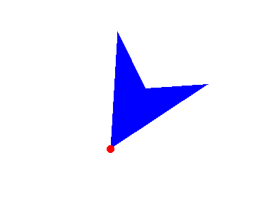
The object we rotate is the arrow. But looking at this code, can you see where the arrow is plotted? Look at line 38 where we call the ARROW function. The ARROW is on line 12. Obviously, the arrow must be somewhere inside the function on line 12, but where? The arrow is defined in lines 14 and 15. Note that we have two arrays to plot this arrow. Here we draw it in a very simple way. Now begins the most interesting part.

This arrow is defined in absolute terms. That is, we plot it as it would be represented in the real world, but we can also represent it virtually. Instead of integer values, you can use floating point values. Thus, by multiplying the values plotting the arrow by any scalar, we can determine its size. However, in order not to complicate the case, we did not do this here. I want to make it as simple as possible so that you, dear readers, can understand how to implement matrix factorization.

There is something in line 16 that may confuse many people. But the reason why it is written that way is easy to understand. Since we don't know in advance how many points we'll use to draw the object, and we need an intermediate array to draw it in line 24, we need to somehow tell the application to allocate memory for us. Using the form in line 16, we tell the compiler that it should allocate as much space as it would take to draw the points. That is, we have a dynamic array that is used, but it is allocated statically. If we didn't use this way of writing code, we would have to create the same code as in the Arrow function, assembled as shown in the code below.

11. //+------------------------------------------------------------------+
12. void Arrow(const int x, const int y, const ushort angle)
13. {
14.     int ax[] = {0, 150, 100, 150},
15.         ay[] = {0, -75,   0,  75};
16.     int dx[], dy[];
17.     
18.     ArrayResize(dx, ax.Size());
19.     ArrayResize(dy, ax.Size());
20.     
21.     for (int c = 0; c < (int)ax.Size(); c++)
22.     {
23.         dx[c] = (int)((ax[c] * cos(_ToRadians(angle))) + (ay[c] * sin(_ToRadians(angle)))) + x;
24.         dy[c] = (int)((ax[c] * (-sin(_ToRadians(angle)))) + (ay[c] * cos(_ToRadians(angle)))) + y;
25.     }
26. 
27.     canvas.FillPolygon(dx, dy, ColorToARGB(clrBlue, 255));
28.     canvas.FillCircle(x, y, 5, ColorToARGB(clrRed, 255));
29. 
30.     ArrayFree(dx);
31.     ArrayFree(dy);
32. }
33. //+------------------------------------------------------------------+

Notice that on line 16, we now have a dynamic array indication. This type of array defines the space that will be used during execution. We need to make the following changes. In lines 18 and 19 of the code, we must allocate the necessary space so that the program does not terminate abnormally during execution. Also, in this code, we have to return the memory allocated in lines 30 and 31 to the operating system, which is considered a good programming practice. Many programmers tend to not return allocated resources, but this makes the application consume resources: the application does not release them, and this makes it difficult to manage. But other than those small differences that you can see between the snippet and the main code, everything else works the same.

Let's get back to the main code now. The loop on line 18 will go through all the points that are part of the shape we want to rotate.

Now pay attention to something interesting. We rotate the shape and move it to a certain place. Specifically, we move it to the X and Y point, which in this case is the center of the screen. Look at line 38 where we define the location and the rotation angle, which is 60 degrees.

Since all trigonometric functions use values in radians by default rather than degrees, we need to convert degrees to radians. This is exactly what is done in the definition of line 10. This way it will be more natural to say how much the shape should rotate, rather than expressing the value in radians, which can be quite confusing in many cases.

So, for each of the points in the array, we apply the formula shown below.

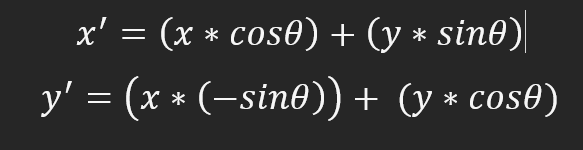
The image will rotate counter-clockwise so that zero degrees corresponds to the nine o'clock position on the clock. To make it clearer, 90 degrees is six hours, 180 degrees is three hours, and 270 degrees is twelve hours. Remember that the rotation is counter-clockwise. To change this behavior, you need to change the calculation method. There is nothing complicated about it, in fact, everything is very simple. To rate clockwise rotation, you will need to change the formula to the one below.

Everything is extremely simple. In this case, three o'clock would be a zero degree angle, six o'clock would be a 90-degree angle, nine o'clock would be a 180-degree angle, and twelve o'clock would be a 270-degree angle. While it looks like we've just changed the angle value from zero to 180 degrees, we've done something more: the direction of rotation has now changed from counter-clockwise to clockwise.

But that's not what I wanted to show. It's just an interesting point. To really explain what I want to show, let's first present everything in the form that everyone usually uses. Precisely because in many cases it is simpler and easier. However, this is not something we can easily adapt to any situation.

Now we will not dwell on this in detail, since the main focus of the article is not on this but on modeling matrix calculations. Let's look at how programmers typically solve these problems. The easiest way is to transform the things we are interested in into virtual units. We first perform all the calculations and then convert the result into graphic units of measurement. When creating something using virtual units, we will use floating values, usually of type double, rather than integers. So the same code we saw before would look like this:

01. //+------------------------------------------------------------------+
02. #property copyright "Daniel Jose"
03. #property indicator_chart_window
04. #property indicator_plots 0
05. //+------------------------------------------------------------------+
06. #include <Canvas\Canvas.mqh>
07. //+------------------------------------------------------------------+
08. CCanvas canvas;
09. //+------------------------------------------------------------------+
10. #define _ToRadians(A) (A * (M_PI / 180.0))
11. //+------------------------------------------------------------------+
12. void Arrow(const int x, const int y, const ushort angle, const uchar size = 100)
13. {
14.     double ax[] = {0.0,  1.5, 1.0, 1.5},
15.            ay[] = {0.0, -.75, 0.0, .75};
16.     int dx[ax.Size()], dy[ax.Size()];
17.     
18.     for (int c = 0; c < (int)ax.Size(); c++)
19.     {
20.         ax[c] *= size;
21.         ay[c] *= size;
22.         dx[c] = (int) ((ax[c] * cos(_ToRadians(angle))) + (ay[c] * sin(_ToRadians(angle)))) + x;
23.         dy[c] = (int) ((ax[c] *(-sin(_ToRadians(angle)))) + (ay[c] * cos(_ToRadians(angle)))) + y;
24.     }
25. 
26.     canvas.FillPolygon(dx, dy, ColorToARGB(clrGreen, 255));
27.     canvas.FillCircle(x, y, 5, ColorToARGB(clrRed, 255));
28. }
29. //+------------------------------------------------------------------+
30. int OnInit()
31. {    
32.     int px, py;
33.     
34.     px = (int)ChartGetInteger(0, CHART_WIDTH_IN_PIXELS, 0);
35.     py = (int)ChartGetInteger(0, CHART_HEIGHT_IN_PIXELS, 0);
36. 
37.     canvas.CreateBitmapLabel("BL", 0, 0, px, py, COLOR_FORMAT_ARGB_NORMALIZE);
38.     canvas.Erase(ColorToARGB(clrWhite, 255));
39.         
40.     Arrow(px / 2, py / 2, 60);
41. 
42.     canvas.Update(true);
43.     
44.     return INIT_SUCCEEDED;
45. }
46. //+------------------------------------------------------------------+
47. int OnCalculate(const int rates_total, const int prev_calculated, const int begin, const double &price[])
48. {
49.     return rates_total;
50. }
51. //+------------------------------------------------------------------+
52. void OnDeinit(const int reason)
53. {
54.     canvas.Destroy();
55. }
56. //+------------------------------------------------------------------+

Almost nothing has changed, except that we can now zoom in on the created object. This is done on lines 20 and 21. The object is created on lines 14 and 15. All code remains virtually unchanged. However, this simple change can help port the application to other scenarios. For example, if the user changes the size of the chart, you can change only the size parameter in line 12 to keep the objects in a certain proportion.

But I still don't understand how this would help me work with matrices. If i can do it like this, why complicate it? Well, let's see if it really is more difficult to do things like this with matrices. For this, we will start a new topic.

Now using matrix factorization

Since the purpose of this article is to educate the reader, I will try to keep things as simple as possible. Therefore, we implement only what is necessary to demonstrate the material we need, that is, matrix multiplication in this particular case. But you, dear readers, will see that even this alone is enough to perform matrix-scalar multiplication. The most significant difficulty that many people encounter when implementing code using matrix factorization is this: unlike scalar factorization, where in almost all cases the order of the factors does not change the result, this is not the case when using matrices. What would the same code as in the previous topic look like if we used matrices? Below is the code where factorization is done using matrices.

01. //+------------------------------------------------------------------+
02. #property copyright "Daniel Jose"
03. #property indicator_chart_window
04. #property indicator_plots 0
05. //+------------------------------------------------------------------+
06. #include <Canvas\Canvas.mqh>
07. //+------------------------------------------------------------------+
08. CCanvas canvas;
09. //+------------------------------------------------------------------+
10. #define _ToRadians(A) (A * (M_PI / 180.0))
11. //+------------------------------------------------------------------+
12. void MatrixA_x_MatrixB(const double &A[][], const double &B[][], double &R[][], const int nDim)
13. {
14.     for (int c = 0, size = (int)(B.Size() / nDim); c < size; c++)
15.     {
16.         R[c][0] = (A[0][0] * B[c][0]) + (A[0][1] * B[c][1]);
17.         R[c][1] = (A[1][0] * B[c][0]) + (A[1][1] * B[c][1]);
18.     }
19. }
20. //+------------------------------------------------------------------+
21. void Arrow(const int x, const int y, const ushort angle, const uchar size = 100)
22. {
23.     double M_1[2][2]{
24.                         cos(_ToRadians(angle)), sin(_ToRadians(angle)),
25.                         -sin(_ToRadians(angle)), cos(_ToRadians(angle))
26.                     },
27.            M_2[][2] {
28.                         0.0,  0.0,
29.                         1.5, -.75,
30.                         1.0,  0.0,
31.                         1.5,  .75
32.                     },
33.            M_3[M_2.Size() / 2][2];
34. 
35.     int dx[M_2.Size() / 2], dy[M_2.Size() / 2];
36.     
37.     MatrixA_x_MatrixB(M_1, M_2, M_3, 2);
38.     ZeroMemory(M_1);
39.     M_1[0][0] = M_1[1][1] = size;
40.     MatrixA_x_MatrixB(M_1, M_3, M_2, 2);
41. 
42.     for (int c = 0; c < (int)M_2.Size() / 2; c++)
43.     {
44.         dx[c] = x + (int) M_2[c][0];
45.         dy[c] = y + (int) M_2[c][1];
46.     }
47. 
48.     canvas.FillPolygon(dx, dy, ColorToARGB(clrPurple, 255));
49.     canvas.FillCircle(x, y, 5, ColorToARGB(clrRed, 255));
50. }
51. //+------------------------------------------------------------------+
52. int OnInit()
53. {    
54.     int px, py;
55.     
56.     px = (int)ChartGetInteger(0, CHART_WIDTH_IN_PIXELS, 0);
57.     py = (int)ChartGetInteger(0, CHART_HEIGHT_IN_PIXELS, 0);
58. 
59.     canvas.CreateBitmapLabel("BL", 0, 0, px, py, COLOR_FORMAT_ARGB_NORMALIZE);
60.     canvas.Erase(ColorToARGB(clrWhite, 255));
61.         
62.     Arrow(px / 2, py / 2, 160);
63. 
64.     canvas.Update(true);
65.     
66.     return INIT_SUCCEEDED;
67. }
68. //+------------------------------------------------------------------+
69. int OnCalculate(const int rates_total, const int prev_calculated, const int begin, const double &price[])
70. {
71.     return rates_total;
72. }
73. //+------------------------------------------------------------------+
74. void OnDeinit(const int reason)
75. {
76.     canvas.Destroy();
77. }
78. //+------------------------------------------------------------------+

We kept the code as simple as possible, without any special modifications, so that you, dear readers, could understand it. Usually when I write factorization using matrix calculations, I do it a little differently, but we will talk about this in future articles, as some details need to be explained. So, I have to explain these details further, and although it may seem simple, if you don't take care of it properly, you will find yourself in a bottomless hole. But what does this crazy code do anyway? It does the same thing as in the previous topic, only here we use matrix multiplication to perform the same calculations. This code may seem very complicated to you, but no, it is much simpler than the previous one. Everything is much simpler if you understand how to multiply one matrix by another. However, the multiplication does not happen quite as expected. In other words, it won't let us do some things if we need to modify the code. But, as I already said, this version is for demonstration purposes only. The correct option will be shown in the next article. However, factorization will give the expected result, even if it is performed in a somewhat strange way.

You should know this detail before using this. But if you already have some idea of how matrix factorization works, the rest will be much easier to understand. Note that line 12 implements the code that performs matrix factorization. Something simple. Basically, we multiply the first matrix by the second and place the result into the third. Since the multiplication is performed for the columns of one matrix by the rows of another, factorization is fairly easy. There are some rules that need to be followed here, for example, the number of rows in one matrix must be equal to the number of columns in the other. This is basic math about matrices, so try to understand it first if you don't know how to proceed or why it needs to be done that way. In matrix A we place columns, and in matrix B we place rows. In our case, we get something equivalent to what you see below.

I know that at first glance it may all seem very confusing, but it is all very simple. The matrix of elements A must be multiplied by the matrix of elements B. As a result, we obtain a matrix of elements R. Basically, it is like this:
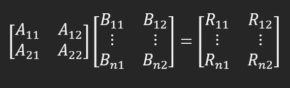
R11 = (A11 x B11) + (A12 x B12);  R12 = (A21 x B11) + (A22 x B12) R21 = (A11 x B21) + (A12 x B22);  R22 = (A21 x B21) + (A22 x B22) R31 = (A11 x B31) + (A12 x B32);  R32 = (A21 x B31) + (A22 x B32)
and so on. Note that this is exactly what would be done if the computations were scalar. This is exactly what the procedure in line 12 does. I think it's important that we have much more freedom in constructing our computations. To understand this, let's look at the function in line 21, where the arrow is constructed and presented. 5 matrices are defined here. We could use less. Let's get this straight first. In the future, we may look at how we can model this in a much more intuitive and understandable way, but even in this model it's still pretty simple to understand. Between lines 23 and 33 we draw our matrices, they will be used in the calculations. Now, on line 35, we declare the ones we will use to represent the arrow on the screen. Between lines 37 and 40 we perform the necessary calculations. Now pay attention: what we are going to do is very interesting. Both from a practical point of view and from the point of view of freedom of factorization. In line 37, we first multiply matrix M_1 by matrix M_2, and the result goes into matrix M_3. What does this multiplication give? The image rotates. However, we cannot yet display it on the screen, since the scale is still used in the model, which is in the M_2 matrix. To represent the image at the correct scale, one more calculation needs to be made. But first, in line 38, we clear the contents of the matrix M_1, and immediately after that, in line 39, we specify how to change the scale of the image. We have a few new options at the moment, but we'll only be focusing on scaling. In line 40, we multiply the object data, which is already rotated, by a new matrix that already contains the desired scale to use. This is shown below.

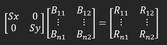
Here Sx is the new dimension along the X axis and Sy is the new dimension along the Y axis. Since we set both values to "Size", the changes will happen as if we are zooming in on the object. That's why I said we can do much more. Since the FillPolygon function doesn't know how to work with this matrix structure, we need to split the data so that FillPolygon can plot the arrow for us. We have a for loop on line 48 and the result is the same as in the previous topic.

Final considerations

In this article, I have presented a fairly simple method for working with matrix calculations. I tried to present something interesting and at the same time find a way to explain in the simplest way how this calculation is done. However, the matrix model considered in this article is not the most suitable one to perform all possible types of factorization. So I will soon publish a new article, in which I will talk about a more suitable model for representing matrices. I will also give an explanation so that you can use this new data factorization method. See you soon in the next article.