Spurious Regressions in Python

Synopsis

Before diving into the realm of algorithmic trading with machine learning, it's crucial to ascertain whether a meaningful relationship exists between the model inputs and the variable we aim to predict. This article illustrates the utility of employing unit root tests on model residuals to validate the presence of such a relationship in our datasets.

Unfortunately, it is possible to construct models using datasets that do not have any genuine relationship. Regrettably these models may yield impressively low error metrics, reinforcing a false sense of control and excessively optimistic outlooks. These flawed models are commonly referred to as "spurious regressions."

This article will begin by first cultivating an intuitive understanding of spurious regressions. Afterwards, we'll generate synthetic time series data to simulate a spurious regression and observe its characteristic effects. Subsequently we'll delve into methods for identifying spurious regressions, relying on our insights to validate a machine learning model crafted in Python. Finally, if our model is validated we will export it to ONNX and implement a trading strategy in MQL5.

Introduction: Spurious Regressions Happen All The Time

During the mid 19th century, Ignaz Semmelweis was a practicing doctor living in Vienna. He was deeply frustrated by the statistics he was observing at the hospital he practiced at.

Fig 1: Ignaz Semmelweis

The problem was that ⅕ healthy women, who gave birth at the hospital, died from fevers contracted during child bearing labor. Ignaz was determined to understand why. Most doctors at the time attributed this to the “bad air” they believed carried evil spirits causing these problems. As comical as this may sound today, it was widely accepted back in its day. But it didn’t satisfy Ignaz. As time elapsed, Ignaz one day observed that doctors and medical students performing autopsies in a mortuary on one side of the hospital would run to deliver babies on the other side of the hospital, without washing their hands in between. After convincing the staff at his local hospital to practice hand hygiene, the maternal mortality rate dropped from 20% to 1%.

Unfortunately, Ignaz’s discoveries went by unnoticed. All efforts he made to share his findings with other doctors and medical institutions only detached him further from the medical community of that time and their concrete belief in “bad air”. Ignaz Semmelweis died a social outcast, in a mental asylum, at the age of 46. What can we learn from the doctors that ignored the wise words Semmelweis offered, and why was it so hard for them to see their mistake?

The problem is that, it is possible to build a model using data that has no relationship whatsoever, furthermore this model may by chance produce low error metrics and falsely prove relationships that do not exist. Such models are called spurious regressions.

A spurious regression is a model that falsely proves a relationship that doesn’t exist. You see, the doctors could’ve told themselves, “There are too many evil spirits in the air today, therefore more mothers will die tomorrow.” As predicted, more women died the following day, however the doctor was right for the wrong reasons. When building machine learning models, our models can also be right for the wrong reasons.

If you are explicitly aware that there is a relationship between your input and the output data, then you have no reason to worry. However, what can you do if you are uncertain? Or if you have never checked and simply assumed there had to be a relationship?

The best known solution, perform specialized tests on the residuals of your model. These tests are called unit root tests. We will not attempt to define unit roots in this discussion, that is another discussion in its own right. However to realize our goals, it is enough to know that if we can find unit roots for our residuals then our regression is spurious.

There is only one material limitation with the unit root solution we are considering today, we may fail to find unit roots though they exist, class 1 error. And alternatively, we may falsely find unit roots that do not exist, a class 2 error.

There are many tests we can use to check if our residuals have unit roots, such as the Augmented Dickey Fuller Test and the Kwiatkowski-Phillips-Schmidt-Shin Test. Each test has its strengths and weakness and will falter under different conditions. In order to see spurious regressions in action, we will generate our own time series data. We will create 2 time series datasets that have no relationship to each other and observe what happens when we train a model using those 2 independent datasets.

Simulating Spurious Regressions

Spurious regressions can happen for a wide variety of reasons, but the most common reason is modelling two independent and non stationary time series. Let us unpack that technical definition. A time series is simply uniformly recorded observations of a random variable. When we say a time series is stationary, its statistical properties, such as mean, variance, and autocorrelation structure, remain relatively constant over time.  A time series is non-stationary when its statistical properties fluctuate over time.

In our discussion, we'll take a hands-on approach by simulating our own data to understand the ground truth at each step. This approach allows us to observe the effects firsthand. We start by importing the necessary packages

import pandas as pd
import numpy as np
import matplotlib.pyplot as plt
import statsmodels.api as sm
from statsmodels.tsa.stattools import adfuller , kpss
from sklearn.linear_model import LinearRegression
from sklearn.metrics import mean_squared_error

Next we will define statistical properties for our two datasets, one will mock our input data and the other our output data. Both datasets will contain random and normally distributed numbers.

size = 1000
mu , sigma = 0 , 1
mu_y , sigma_y = 2 , 4

The code below generates two time series, x_non_stationary and y_non_stationary, representing random walks. The randomness is introduced through the normal distribution, and the cumulative sum ensures that each value in the series depends on the previous values, creating a dynamic, non-stationary behavior.

Both x_non_stationary and y_non_stationary data set is being randomly generated by the numpy.random.normal function. Therefore, there is no relationship between the two datasets.

steps = np.random.normal(mu,sigma,size)
steps_y = np.random.normal(mu_y,sigma_y,size)
x_non_stationary =  pd.DataFrame(100 + np.cumsum(steps),index= np.arange(0,1000))
x_non_stationary_lagged = x_non_stationary.shift(1)
x_non_stationary_lagged.dropna(axis=0,inplace=True)
y_non_stationary =   pd.DataFrame(100 + np.cumsum(steps_y),index= np.arange(0,1000))

Let us see our two random datasets.

plt.plot(x_non_stationary)

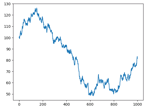
Fig 2: Random walk x

Let us plot our non-stationary y time-series.

plt.plot(y_non_stationary)

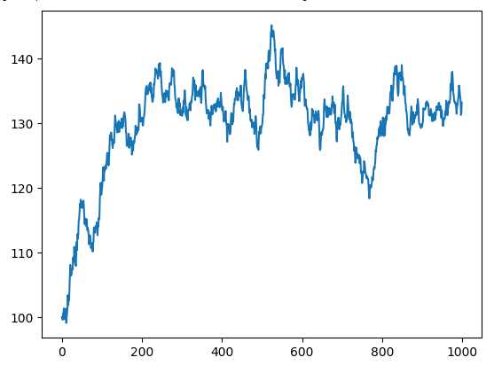
Fig 3: Random walk y.

Now let us observe the results of regressing the two independent and non-stationary time-series.

ols = sm.OLS(y_non_stationary,x_non_stationary)
lm = ols.fit()
print(lm.summary())

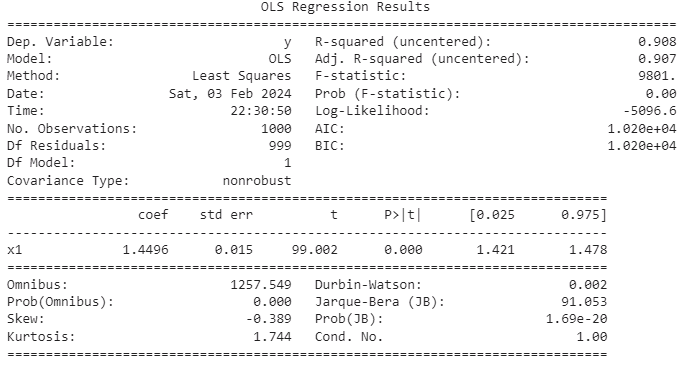
Fig 4:  The Summary Results of Regressing Two Independent Non-Stationary Variables.

In many time series, there is a random trend component known as the stochastic trend. Even when two time series are independent, their stochastic trends may exhibit brief, local correlations. Unfortunately, these momentary correlations can sometimes mislead our models into erroneously concluding that a relationship exists between two independent time series. Spurious regressions arising from such cases often yield high R-squared metrics. It's crucial to remember that R-squared measures the proportion of variance in the response explained by variance in the independent variables. Therefore, if two variables have correlated stochastic trends, the reliability of the R-squared metric may be compromised. The issue of spurious regression is particularly relevant in the context of time-series data and warrants careful consideration.

Our model has an Adjusted R-squared metric that nearly reaches 1, signifying that the model perceives the fit as nearly perfect. The model asserts that approximately 90% of the variation in the response variable can be explained by the variance in the predictors. However, this demonstration serves as a crucial reminder of the pitfalls associated with spurious regressions. We know that there is no relationship between inputs and outputs, they are both random with nothing in common.

The challenges persist as the P value appears significant, and 0 is conspicuously absent from our confidence intervals. While this might typically be interpreted as a hallmark of a superb fit, caution is warranted. The model, in this case, erroneously indicates a strong relationship that does not actually exist. We created the input and output data ourselves, therefore we know there is no relationship.

Lagging The Predictor

A telltale sign of a spurious regression emerges when we include a lagged version of the predictor. In such cases, the once-significant coefficient suddenly becomes insignificant, as we will soon observe. This phenomenon serves as a crucial indicator, guiding us away from erroneous conclusions and highlighting the importance of understanding and addressing spurious regressions in time series analysis.

We will repeat the same procedure as above, however this time we will also include a lagged version of the input data.

ols = sm.OLS(y_non_stationary.iloc[0:998,0],x_matrix.loc[0:998,['current_x','lagged_x']])
lm = ols.fit()
print(lm.summary())

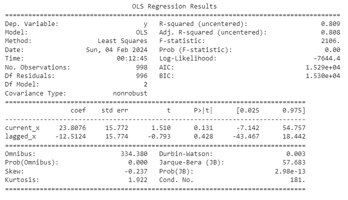
Fig 5: Summary statistics from our spurious regression.

Adding another layer of caution, observe that our R-squared value surpasses our Durbin-Watson value. This observation can be considered an additional red flag pointing towards a potential spurious regression. The Durbin-Watson statistic, employed in regression analysis, serves to detect the presence of autocorrelation in the residuals of a regression model. Autocorrelation manifests when the residuals in a time series or regression model exhibit correlation with each other. In the context of time-series data, where observations are dependent on previous ones, the Durbin-Watson test becomes particularly relevant. Its results provide valuable insights into the presence of autocorrelation, further guiding us in our interpretation of the model's performance.

Durbin-Watson Statistic

•     Range: The Durbin-Watson statistic has values between 0 and 4.
•     Interpretation: A value close to 2 indicates no significant autocorrelation. Values significantly below 2 suggest positive autocorrelation (residuals are positively correlated). Values significantly above 2 suggest negative autocorrelation (residuals are negatively correlated).

While a high R-squared and a low Durbin-Watson value may raise suspicions of spurious regression, it's important to note that these indicators alone do not conclusively confirm its presence. In the realm of time series analysis, additional diagnostic tests and domain knowledge become essential components of a thorough assessment. 

Unit Root Tests

The most reliable method for identifying a spurious regression lies in the analysis of the residuals. If the residuals of our model lack stationarity, it provides a strong indication that the regression is indeed spurious. However, determining whether a given time series is stationary is not a straightforward task. In our case, knowing that the regression is spurious and, therefore, the residuals are non-stationary, the Augmented Dickey Fuller Test may fail to reject the null hypothesis. In other words, it may fail to demonstrate that the data is not stationary even though the regression is spurious, illustrating the subtleties and challenges involved in identifying spurious regressions. This underscores the importance of a nuanced approach, combining statistical tests and domain knowledge to navigate the intricacies of time series analysis effectively.

We will now use sklearn to fit a model on our training set.

lm = LinearRegression()
lm.fit(x[train_start:train_end],y[train_start:train_end])

We will then calculate the residuals.

residuals = y[test_start:test_end] - lm.predict(x[test_start:test_end])

Let us plot the residuals.

residuals.plot()

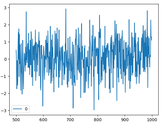
Fig 6: The Residuals of Our Regression Model Built With Scikit-Learn.

Now, we will subject our residuals to the Augmented Dickey-Fuller Test to determine their stationarity.

Augmented Dickey-Fuller Test

The Augmented Dickey-Fuller (ADF) test serves as a pivotal statistical instrument designed for the evaluation of time series stationarity or the identification of a unit root, indicative of non-stationarity. Within the domain of time series analysis, stationarity assumes a paramount role, signifying the constancy of statistical attributes like mean and variance over time. The presence of a unit root in a time series, denoting non-stationarity, prompts a reasonable suspicion that observations within the time series may be characterized as stochastic or random in nature. The ADF test, therefore, offers a robust methodology for scrutinizing the temporal behavior of a dataset, contributing to a nuanced understanding of its inherent characteristics and potential implications for subsequent analyses.

1. Null Hypothesis: The null hypothesis of the ADF test posits that the time series possesses a unit root, indicating non-stationarity.
2. Alternative Hypothesis: The alternative hypothesis of the Augmented Dickey-Fuller (ADF) test is that the time series does not have a unit root and is stationary.
3. The Decision Rule: The decision rule in the ADF test involves comparing the test statistic to critical values. If the test statistic is less than the critical value, the null hypothesis (presence of a unit root) is rejected, indicating stationarity. Conversely, if the test statistic is greater than the critical value, there is insufficient evidence to reject the null hypothesis, suggesting non-stationarity.

As we undertake the Augmented Dickey-Fuller (ADF) test on the residuals generated from our model, the resultant findings will serve as a crucial determinant in discerning the presence of stationarity or non-stationary characteristics within the residuals. The ADF test holds significant importance in the validation process of our regression results, playing a pivotal role in ensuring the reliability of our analytical framework. By elucidating the stationarity properties of the residuals, this test contributes substantially to the enhancement of the interpretative robustness of our time series analysis.

adfuller(residuals)

(-12.753804093890963, 8.423533501802878e-24, 2, 497, {'1%': -3.4435761493506294, '5%': -2.867372960189225, '10%': -2.5698767442886696}, 1366.9343966932422)

Our primary focus lies on the p-value derived from this experiment, specifically the second value in the provided list, which is 8.423533501802878e-24. Notably, this p-value approaches zero and significantly surpasses any reasonable critical value. In the context of the Augmented Dickey-Fuller (ADF) test, if the ADF statistic is less than the critical value, rejecting the null hypothesis becomes pertinent, signifying the presence of stationarity.

It is imperative to acknowledge that the ADF test, akin to any statistical test, is accompanied by inherent limitations and assumptions. There exist various factors that can contribute to the failure of the ADF test in accepting the null hypothesis, thereby leading to the rejection of the presence of a unit root, even when the underlying data is non-stationary. Understanding these nuances is crucial for a comprehensive interpretation of the test results.

1. Small Sample Size: The ADF test performance may be affected by small sample sizes. In such cases, the test might lack sufficient power to detect non-stationarity.
2. Poor Lag Order: The choice of lag order in the ADF test is crucial. If the lag order is incorrectly specified, it can lead to inaccurate results. Using too few or too many lags may impact the test's ability to capture the underlying structure of the data.
3. Presence of Deterministic Trends: If the data contains deterministic trends (e.g., linear trends, quadratic trends) that are not accounted for in the test model, the ADF test might fail to reject the null hypothesis. In such cases, pre-processing steps like detrending might be necessary.
4. Inadequate Differencing: If the differencing order used in the ADF test is insufficient to make the data stationary, the test might fail to reject the null hypothesis.

Kwiatkowski-Phillips-Schmidt-Shin

The Kwiatkowski-Phillips-Schmidt-Shin (KPSS) test stands as a viable alternative to the Augmented Dickey-Fuller (ADF) test for evaluating the stationarity of time series data. While both tests are prevalent in time series analysis, they diverge in their null and alternative hypotheses, as well as their underlying models. The selection between the ADF and KPSS tests is contingent upon the specific characteristics of the time series under examination and the overarching research inquiry. Leveraging both tests in tandem often provides a more comprehensive analysis of stationarity, offering researchers a nuanced understanding of the time series dynamics.

1. Null Hypothesis: The null hypothesis of the KPSS test is that the time series is trend-stationary. Trend-stationarity implies that the series exhibits a unit root, suggesting the presence of a deterministic trend.
2. Alternative Hypothesis: The alternative hypothesis of the KPSS test is that the time series is not trend-stationary, indicating it is difference-stationary or stationary around a stochastic trend.
3. The Decision Rule: The decision rule for the KPSS test involves comparing the test statistic to critical values at a chosen significance level (e.g., 1%, 5%, or 10%). If the test statistic is greater than the critical value, the null hypothesis is rejected, suggesting that the time series is not trend-stationary. On the other hand, if the test statistic is smaller than the critical value, the null hypothesis cannot be rejected, implying trend-stationarity.

In the case of the KPSS test, a commonly adopted threshold is a significance level of 0.05. If the KPSS statistic falls below this threshold, it suggests non-stationarity in the data. In our analysis, the KPSS statistic yielded a value of 0.016, affirming its deviation from the critical threshold and indicating a tendency towards non-stationarity in the dataset. This outcome further underscores the importance of considering multiple diagnostic tools, such as both the ADF and KPSS tests, to ensure a thorough and accurate assessment of the time series characteristics.

kpss(residuals)

(0.6709994557854182, 0.016181867655871072, 1, {'10%': 0.347, '5%': 0.463, '2.5%': 0.574, '1%': 0.739})

The KPSS test may falsely reject the null hypothesis (H0) under certain circumstances, leading to a Type I error. A Type I error occurs when the test incorrectly concludes that the time series is not trend-stationary when, in reality, it is.

Here are some situations where the KPSS test might incorrectly reject the null hypothesis:

1. Seasonal Patterns: The KPSS test is sensitive to both trend and seasonality. If a time series exhibits a strong seasonal pattern, the test may interpret it as a non-stationary trend. In such cases, differencing might be necessary to address the seasonality.
2. Structural Breaks: If there are structural breaks in the time series, such as sudden and significant changes in the underlying data-generating process, the KPSS test may detect these as non-stationary trends. Structural breaks can lead to a rejection of the null hypothesis.
3. Outliers: The presence of outliers in the data can influence the performance of the KPSS test. Outliers might be perceived as trend deviations, leading to a rejection of trend-stationarity. Robustness to outliers is an important consideration when interpreting the results of the KPSS test.
4. Nonlinear Trends: The KPSS test assumes a linear trend. If the underlying trend in the time series is nonlinear, the test may produce misleading results. Nonlinear trends may not be adequately captured by the test, leading to a false rejection of stationarity.

It's crucial to interpret the results of the KPSS test cautiously and consider the specific characteristics of the time series being analyzed. Additionally, combining the KPSS test with other stationarity tests, such as the Augmented Dickey-Fuller (ADF) test, can provide a more comprehensive assessment of the stationarity properties of the time series.

Putting it All Together

Having established a foundation of confidence, it is now opportune for us to transition our focus away from synthetic control data and redirect our efforts toward the analysis of authentic market data sourced directly from our MetaTrader 5 Terminal. To facilitate this transition, we propose the development of a MetaQuotes Language 5 (MQL5) script. This script will be specifically designed to retrieve data from our trading terminal, formatting and exporting it into CSV format.

Commencing our script, the initial step involves the declaration of global variables, with the first set dedicated to housing the handles of our technical indicators. These variables will play a pivotal role in efficiently managing and accessing the relevant indicators throughout the script execution, contributing to the overall coherence and organization of our MetaQuotes Language 5 (MQL5) program.

//---Our handlers for our indicators
int ma_handle;
int rsi_handle;
int cci_handle;
int ao_handle;

Subsequently, we need data structures meticulously designed to accommodate and organize the readings from our technical indicators. These data structures will be used throughout the script execution. 

//---Data structures to store the readings from our indicators
double ma_reading[];
double rsi_reading[];
double cci_reading[];
double ao_reading[];

Following naturally afterwards, we create a name for the file.

//---File name
string file_name = "Market Data.csv";

Now we will define how much data to fetch.

//---Amount of data requested
int size = 3000;

Commencing the development of our OnStart event handler, the first call to order involves the initialization of our designated technical indicators.

//---Setup our technical indicators
ma_handle = iMA(_Symbol,PERIOD_CURRENT,20,0,MODE_EMA,PRICE_CLOSE);
rsi_handle = iRSI(_Symbol,PERIOD_CURRENT,60,PRICE_CLOSE);
cci_handle = iCCI(_Symbol,PERIOD_CURRENT,10,PRICE_CLOSE);
ao_handle = iAO(_Symbol,PERIOD_CURRENT);

Proceeding with the script execution, the subsequent task entails the transfer of values from our indicator handles to the corresponding data structures. This essential process involves a meticulous mapping of indicator outputs to the pre-established data structures.

//---Set the values as series
CopyBuffer(ma_handle,0,0,size,ma_reading);
ArraySetAsSeries(ma_reading,true);
CopyBuffer(rsi_handle,0,0,size,rsi_reading);
ArraySetAsSeries(rsi_reading,true);
CopyBuffer(cci_handle,0,0,size,cci_reading);
ArraySetAsSeries(cci_reading,true);
CopyBuffer(ao_handle,0,0,size,ao_reading);
ArraySetAsSeries(ao_reading,true);

As we prepare to initiate the file-writing process, a critical precursor involves the establishment of a file handler within our script.

//---Write to file
int file_handle=FileOpen(file_name,FILE_WRITE|FILE_ANSI|FILE_CSV,",");

Subsequently, a pivotal phase in our script unfolds as we systematically traverse through the dataset, orchestrating the meticulous process of writing data to our designated CSV file. This iterative procedure involves a detailed examination and extraction of each data point, adhering to a carefully orchestrated sequence that aligns with the established parameters.

for(int i=-1;i<=size;i++){
      if(i == -1){
            FileWrite(file_handle,"Open","High","Low","Close","MA 20","RSI 60","CCI 10","AO");
      }
      
        else{
                FileWrite(file_handle,iOpen(_Symbol,PERIOD_CURRENT,i),
                                        iHigh(_Symbol,PERIOD_CURRENT,i),
                                        iLow(_Symbol,PERIOD_CURRENT,i),
                                        iClose(_Symbol,PERIOD_CURRENT,i),
                                        ma_reading[i],
                                        rsi_reading[i],
                                        cci_reading[i],
                                        ao_reading[i]);
      } 
}

Following the completion of the script setup, proceed to execute the script on the symbol of your preference. Subsequently, the script will generate a CSV file, mirroring the format exemplified below, thereby providing a comprehensive and structured representation of the pertinent data associated with the selected symbol.

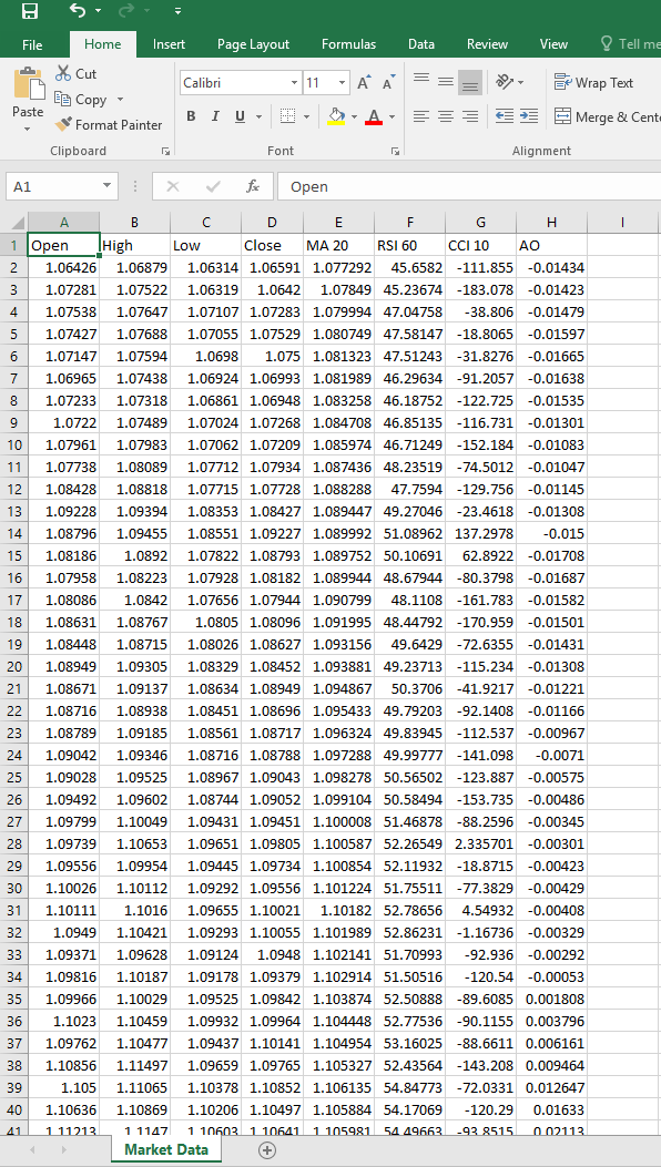
Fig 7:Our Market Data CSV File.

With our focus now shifted towards the analysis of authentic market data, our objective is to construct a regression model designed to predict the anticipated price growth within the subsequent 15 minutes. The pivotal criterion for our analytical pursuit is the validation of the regression model's authenticity. Once this authenticity is established, we intend to export the validated model to ONNX format, subsequently leveraging it for the development of an Expert Advisor.

Commencing this phase, our initial step involves the loading of essential dependencies. Among these dependencies, a notable addition is the 'Arch' package, renowned for its comprehensive suite of statistical analysis tools. The integration of 'Arch' furnishes us with an array of invaluable resources to employ in our analytical endeavors, enhancing the depth and sophistication of our approach to market data analysis.

import pandas as pd
import numpy as np
import statsmodels.api as sm
import matplotlib.pyplot as plt
from sklearn.linear_model import LinearRegression
from sklearn.metrics import mean_squared_error
from arch.unitroot import PhillipsPerron , ADF , KPSS
import onnx
from skl2onnx import convert_sklearn
from skl2onnx.common.data_types import DoubleTensorType

Then we read in the csv we created using our MQL5 script.

csv = pd.read_csv("/enter/your/path/here")

We then prepare our target, our target is the growth in the close price.

csv["Target"] = csv["Close"] / csv["Close"].shift(-15)
csv.dropna(axis=0,inplace=True)

We can examine our data frame.

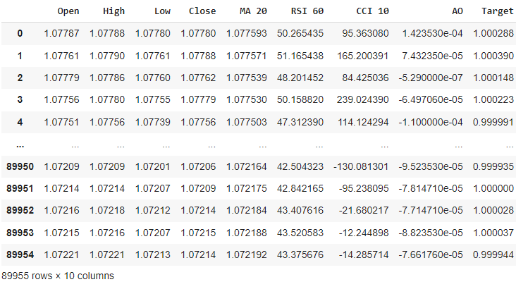
Fig 8: Reading in Our Market Data CSV File With Pandas

From there we will prepare our train-test split

train = np.arange(0,20000)
test = np.arange(20020,89984)

We will now fit a multiple linear regression using statsmodels.

ols = sm.OLS(csv.loc[:,"Target"],csv.loc[:,["Open","High","Low","Close","MA 20","RSI 60","CCI 10","AO"]])
lm = ols.fit()
print(lm.summary())

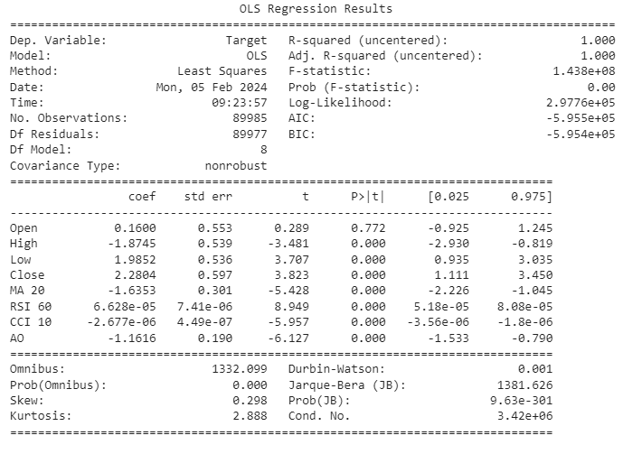
Fig 9:Results of Regressing All The Variables To Predict The Growth in Price.

Allow us to collectively delve into the interpretation of our model results. The confidence interval for the coefficient associated with the Open price feature encompasses 0, implying a lack of statistical significance. Consequently, the decision to exclude this feature from our model is informed by the potential insignificance of its contribution. Further scrutiny reveals that both the Relative Strength Index (RSI) and the Commodity Channel Index (CCI) exhibit coefficients in close proximity to 0, with their respective confidence intervals exhibiting a similar proximity to this value. Given this, we exercise prudence in opting to eliminate these features, positing that their marginal contribution to informativeness may be limited.

Although our model boasts a notably high R-squared value, suggesting a substantial proportion of the variance is explained by the included features, a concomitant examination of the Durbin-Watson (DW) statistic reveals a low value. This prompts a circumspect approach, as the low DW statistic indicates the possibility of residual correlation, which could compromise the validity of our model. Consequently, we advocate for a meticulous analysis of the residuals, specifically focusing on their stationarity. This additional layer of scrutiny is imperative for ensuring the robustness and reliability of our model in capturing the underlying patterns in the data.

Let's create a data structure to store the features we think may be important.

predictors = ["High","Low","Close","MA 20","AO"]

Let's record the residuals.

residuals = csv.loc[test[0]:test[-1],"Target"] - lm.predict(csv.loc[test[0]:test[-1],predictors])

Let us proceed with the generation of residual plots, a critical step in the model evaluation process. 

plt.plot(residuals)

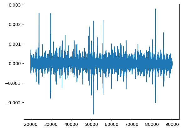
Fig 10: Plotting The Residuals From Forecasting Market Data.

Analyzing residuals is a crucial step in understanding how well our model fits the data. Residuals can reveal if our model has any systematic errors or if it's making consistent mistakes. This is important because it helps us check if our model follows certain basic rules, like having consistent variation in its predictions and not relying on previous errors.

One thing we need to watch out for when looking at residuals is something called a "unit root." This basically means that the residuals show a pattern of change over time that doesn't go away. It's like having a persistent trend in our errors. Finding a unit root in residuals is a big deal because it messes with some of the basic assumptions we make about our model, like that each prediction is independent from the others.

Dealing with unit roots is important because if we don't, it can mess up our estimates of how good our model is and make it harder to trust the conclusions we draw from it.

So, when we dig into residuals, we're not just checking boxes. We're making sure our model holds up under scrutiny and fixing any issues, like unit roots, to make our predictions more reliable.

It may help to think of it this way: Imagine the task of classifying a cat, a seemingly straightforward endeavor. In an ideal scenario, where our comprehension of a cat symbolizes an unchanging truth, each classification would be flawless, if we plotted the error from such an ideal model we would obtain stationary and straight line, represented by y = a constant. This line symbolizes the constancy of the truth that a cat is always a cat at all points in time and if we called it a cat at any point in time our error would be 0.

However, if the classifier's proficiency diminishes, introducing misclassifications that cause the residuals to deviate from this state of perfect stationarity. This deviation corresponds to the classifier's divergence from the truth and manifests as fluctuations in the residuals. The nonstationarity arises on days when a dog might be mislabeled as a cat or vice versa, reflecting the classifier's uncertain grasp on the defining characteristics of a cat.

To delve deeper into statistical rigor, consider the link between a unit root in residuals and non-stationarity in time series analysis. The presence of a unit root in residuals, analogous to a classifier's lack of knowledge, signifies non-stationarity, leading to increased volatility in the residuals. The more profound the lack of knowledge, the more pronounced the fluctuations become, akin to misclassifying dogs as cats and vice versa.

Understanding these concepts is important because it helps us fine-tune our model to make better predictions. So, even if things look good at first glance, it's worth double-checking to make sure our residuals are behaving as they should. Remember, there's no one-size-fits-all test for this, so it's best to use multiple methods and look at the overall trends in our residuals.

Phillip-Perron Test

The Phillips-Perron Test is a statistical test used in econometrics and time series analysis to assess the presence of a unit root in a time series dataset. A unit root implies that a time series variable has a stochastic trend, making it non-stationary. Stationarity is a crucial assumption in many statistical analyses, and non-stationary time series data can lead to spurious regression results.

The Phillips-Perron Test is a variation of the Dickey-Fuller test, and it was proposed by Peter C.B. Phillips and Pierre Perron in 1988. Like the Dickey-Fuller test, the Phillips-Perron Test is designed to detect the presence of a unit root by examining the behavior of a time series variable over time.

The basic idea behind the Phillips-Perron Test is to regress the differenced time series variable on its lagged values. The test statistic is then used to evaluate whether the coefficient on the lagged variable is significantly different from zero. If the coefficient is significantly different from zero, it suggests evidence against the presence of a unit root and implies that the time series is stationary.

One notable feature of the Phillips-Perron Test is that it allows for certain forms of serial correlation and heteroscedasticity in the data, which the original Dickey-Fuller test does not account for. This makes the Phillips-Perron Test robust to certain violations of assumptions that might be present in real-world time series data.

1. Null Hypothesis: The null hypothesis of the Phillips-Perron Test is that the time series variable contains a unit root, implying that it is non-stationary.
2. Alternative Hypothesis: The alternative hypothesis is that the time series variable does not contain a unit root, indicating that it is stationary.
3. Decision Rule: If the computed test statistic is less than the critical value, reject the null hypothesis that a unit root is present, suggesting evidence that the time series is stationary.  If the computed test statistic is greater than the critical value, fail to reject the null hypothesis, indicating insufficient evidence to conclude that the time series is stationary.

We will use the arch library to perform the Phillip-Perron Test.

pp = PhillipsPerron(residuals)

We can obtain summary results. Summary Statistics From The Phillips-Perron Test

pp.summary()

Phillips-Perron Test
(Z-tau)

Test Statistic -73.916

P-value 0.000

Lags 62

Trend: Constant
Critical Values: -3.43 (1%), -2.86 (5%), -2.57 (10%)

Null Hypothesis: The process contains a unit root.
Alternative Hypothesis: The process is weakly stationary.

Let's interpret the results together. The test statistic is -73.916. This value represents how many standard deviations the estimated coefficient is away from the hypothesized value of 1 (indicating the presence of a unit root). In this case, a very large negative test statistic suggests strong evidence against the presence of a unit root, supporting the stationarity of the time series.

The p-value associated with the test statistic is 0.000. The p-value is a measure of the evidence against the null hypothesis. A p-value of 0.000 means that the observed test statistic is extremely unlikely under the assumption that the null hypothesis is true. In practical terms, this extremely small p-value provides strong evidence against the presence of a unit root.

Given the very low p-value (0.000), you would typically reject the null hypothesis at conventional levels of significance (e.g., 0.05). The evidence suggests that the time series is likely stationary, as the p-value is below the chosen significance level. In summary, based on the provided results, you have strong evidence to reject the null hypothesis of a unit root, indicating that the time series is likely stationary. However we cannot base our decisions on test, we want to observe measueres of central tendency from different tests.

Augmented Dickey–Fuller Test

We will use the arch libray to perform the Augmented Dickey-Fuller Test

adf = ADF(residuals)

We can fetch summary statistics. Summary Statistics From The Augmented Dickey Fuller Test

adf.summary()
Augmented Dickey-Fuller Results

Test Statistic -31.300
P-value 0.000
Lags 60

Trend: Constant
Critical Values: -3.43 (1%), -2.86 (5%), -2.57 (10%)

Null Hypothesis: The process contains a unit root.
Alternative Hypothesis: The process is weakly stationary.

Let's now interpret the results. The test statistic is -31.300. Like the Phillips-Perron Test, the ADF test statistic is used to evaluate the presence of a unit root in the time series. In this case, the very large negative value indicates strong evidence against the null hypothesis of a unit root, supporting the idea that the time series is stationary.

The associated p-value is 0.000. Similar to the Phillips-Perron Test, a p-value of 0.000 means that the observed test statistic is extremely unlikely under the assumption that the null hypothesis (presence of a unit root) is true. The very small p-value provides strong evidence against the null hypothesis.

Given the low p-value (0.000), you would typically reject the null hypothesis at conventional levels of significance. The evidence from the Augmented Dickey-Fuller test supports the conclusion that the time series is likely stationary.

Both the Phillips-Perron Test and the Augmented Dickey-Fuller test have provided strong evidence against the presence of a unit root, indicating that the time series is likely stationary. The similarity in results between these two tests is expected, as they are both designed to assess stationarity in time series data. The choice between them often depends on the specific characteristics of the data and the assumptions of the tests. In your case, both tests suggest that the time series is stationary.

Let's export our model to Open Neural Network Exchange Format

ONNX, or Open Neural Network Exchange, is an open and interoperable format for representing machine learning models. Developed by a collaborative community, ONNX enables the seamless exchange of models between various frameworks and tools, fostering interoperability in the machine learning ecosystem. It provides a standardized way to represent and transfer trained models, making it easier for developers to deploy models across different platforms and integrate them into diverse applications. ONNX supports a wide range of machine learning models and frameworks, promoting flexibility and efficiency in model development and deployment workflows.

This code is defining an initial type for a variable named 'double_input' that will be used in the context of generating an ONNX (Open Neural Network Exchange) file. The specified type is 'DoubleTensorType,' indicating that the input data is expected to be in double precision. The shape of the input tensor is determined by the number of columns in a DataFrame (presumably named 'csv') corresponding to the features used for prediction (retrieved using 'csv.loc[:, predictors].shape[1]'). The 'None' in the shape indicates that the size of the first dimension (likely representing the number of instances or samples) is not fixed at this stage.

initial_type_double = [('double_input', DoubleTensorType([None, csv.loc[:,predictors].shape[1]]))]

This code is utilizing the 'convert_sklearn' function to convert our trained linear regression model ('lm') into its ONNX representation. The 'initial_type_double' variable, defined in the previous code snippet, specifies the expected type for the input data as double precision. Additionally, the 'target_opset' parameter is set to 12, indicating the desired version of the ONNX operator set. The resulting 'onnx_model_double' will be an ONNX model representation of the provided linear regression model, suitable for deployment and interoperability with other frameworks that support the ONNX format.

onnx_model_double = convert_sklearn(lm, initial_types=initial_type_double, target_opset=12)

This code is specifying the filename ("EURUSD_ONNX") for saving the ONNX model representation of a linear regression model. The resulting ONNX model, converted using the previously mentioned 'convert_sklearn' function, will be stored with this filename, making it easily identifiable and accessible for future use or deployment.

onnx_model_filename = "EURUSD_ONNX"

This code is combining the previously defined filename ("EURUSD_ONNX") with the suffix "_Double.onnx" to create a new filename ("EURUSD_ONNX_Double.onnx"). Subsequently, the 'onnx.save_model' function is employed to save the ONNX model ('onnx_model_double') to a file with the constructed filename. This process ensures that the ONNX model, representing the linear regression model in double precision, is stored and can be easily referenced using the specified filename.

onnx_filename=onnx_model_filename+"_Double.onnx"
onnx.save_model(onnx_model_double, onnx_filename)

Constructing an Expert Advisor For Our ONNX File in MetaQuotes Language 5 (MQL5) Utilizing The Integrated And Versatile MetaEditor.

Developing an Expert Advisor (EA) for our ONNX file in MetaQuotes Language 5 (MQL5) involves leveraging the capabilities of the integrated and versatile MetaEditor. An Expert Advisor is a script written in MQL5 that enables automated trading within the MetaTrader 5 platform. In this context, the EA will interface with the ONNX file, facilitating seamless integration of machine learning models into trading strategies, thereby enhancing decision-making processes based on predictive analytics. The MetaEditor provides a comprehensive environment for coding, testing, and optimizing EAs, ensuring efficient deployment and execution within the MetaTrader 5 framework.

We first include the Trade library in MQL5, which is a standard library for handling trading operations within MetaTrader 5 (MT5). The Trade library provides predefined functions and structures that facilitate the execution of various trading activities, such as opening and closing positions, managing orders, and handling trade-related events. Including this library in an Expert Advisor (EA) allows for streamlined and efficient implementation of trading logic and operations within the MQL5 code.

//Our trade class helps us open trades
#include <Trade\Trade.mqh>
CTrade Trade;

This code snippet in MQL5 involves the utilization of an Expert Advisor (EA) and incorporates an ONNX model for predictive analytics. The #resource directive is employed to embed the ONNX model file, "EURUSD_ONNX_Double.onnx," into the EA's resources as a byte array named ONNXModel. This facilitates easy access and utilization of the machine learning model within the EA.

The variable ONNXHandle is initialized as INVALID_HANDLE, indicating that it will be used to store the handle or identifier associated with the ONNX model once it is loaded during the execution of the EA.

Additionally, PredictedMove is initialized to -1, suggesting that the predicted move or outcome based on the ONNX model is not yet determined. This variable is likely to be updated with the predicted value once the EA processes relevant data through the ONNX model during its execution. The specifics of the predictive logic and further processing will depend on the subsequent sections of the EA code.

//Loading our ONNX model
#resource "ONNX\\EURUSD_ONNX_Double.onnx" as uchar EURUSD_ONNX_MODEL[]
long     ONNXHandle=INVALID_HANDLE;

In this section of MQL5 code for an Expert Advisor, two sets of variables are declared: ma_handle and ma_reading[] for a moving average, and ao_handle and ao_reading[] for an Awesome Oscillator.

The variable ma_handle serves as a reference or identifier for the moving average indicator, allowing the EA to interact with and retrieve information about this specific technical analysis tool. The array ma_reading[] is intended to store the calculated values of the moving average, enabling the EA to access and analyze its historical values for decision-making.

Similarly, the variable ao_handle is expected to represent an identifier for the Awesome Oscillator indicator, while the array ao_reading[] is designated to store the corresponding calculated values. 

//Handles for our technical indicators and dynamic arrays to store their readings
int ma_handle;
double ma_reading[];
int ao_handle;
double ao_reading[];

//Inputs
int input sl_width = 150; //How wide should the stoploss be?
int input  positions = 1; //How many positions should the we open?
int input lot_multiple = 1; //How many times greater than minimum lot should each position be?

//Symbol variables
double min_volume;
double bid,ask;

//We'll use this time stamp to keep track of the number of candles passing
static datetime time_stamp;

//Our model's forecast will be stored here
vector model_forecast(1);

OnInit Function

The OnInit() function is a crucial part of an Expert Advisor (EA) in MQL5 and serves as the initialization function that is automatically executed when the EA is attached to a chart in MetaTrader 5. In this function, various tasks related to the setup and preparation of the EA are typically performed. The rest of the code we will examine is nested within our OnInit() Handler.

This conditional statement within the Expert Advisor's OnInit() function checks whether the trading symbol is "EURUSD" and the chart timeframe is set to M1 (one-minute intervals). If the conditions are not met, the EA prints a message to the console using the Print() function, stating that the model must specifically operate with the "EURUSD" currency pair on the one-minute timeframe. Subsequently, the return(INIT_FAILED) statement is employed to terminate the EA's initialization process, indicating a failure to initialize if the specified conditions are not satisfied.

int OnInit(){
    //Validating trading conditions
   if(_Symbol!="EURUSD" || _Period!=PERIOD_M1)
     {
      Print("Model must work with EURUSD on the M1 timeframe");
      return(INIT_FAILED);
     }

This code segment within the Expert Advisor (EA) in MQL5 is responsible for creating an ONNX model from a static buffer. The function OnnxCreateFromBuffer is utilized for this purpose, taking as parameters the ONNX model data stored in the ONNXModel buffer and using the default settings for model creation.

Upon execution, the ONNXHandle variable is assigned the handle or identifier associated with the created ONNX model. Subsequently, a conditional statement checks whether the ONNXHandle is a valid handle (not equal to INVALID_HANDLE). If the handle is not valid, the EA prints an error message to the console using the Print() function, providing information about the encountered error (via GetLastError()), and then signals an initialization failure by returning INIT_FAILED.

This code section is crucial for initializing the EA with a functional ONNX model, ensuring that the model is successfully created from the provided buffer. Any failure in this process is promptly communicated.

ONNXHandle=OnnxCreateFromBuffer(ONNXModel,ONNX_DEFAULT);

if(ONNXHandle==INVALID_HANDLE)
{
   Print("OnnxCreateFromBuffer error ",GetLastError());
   return(INIT_FAILED);
}

The line of code declares a constant array named input_shape with two elements. This array is denoted as long and holds integers. The elements of the array represent the shape of input data for a machine learning model or algorithm. In this specific case, the array input_shape is initialized with the values {1, 5}, indicating that the input data is expected to have dimensions of one row and five columns.

//Defining the model's input shape
const long input_shape[] = {1,5};

This code block, within the Expert Advisor in MQL5, checks whether the setting of the input shape for the ONNX model is successful using the function OnnxSetInputShape. The input shape is specified by the input_shape array, which denotes the expected dimensions of the input data.

The if statement evaluates whether the negation of the condition OnnxSetInputShape (returning true if the setting is not successful) holds. If the condition is true, the EA prints an error message to the console using the Print() function, conveying details about the encountered error obtained through GetLastError(). Subsequently, the function returns INIT_FAILED, indicating an initialization failure.

if(!OnnxSetInputShape(ONNXHandle,ONNX_DEFAULT,input_shape)) 
{
    Print("OnnxSetInputShape error ",GetLastError());
    return(INIT_FAILED); 
}

This line of code declares a constant array named output_shape with two elements. Similar to the previous declaration for input_shape, this array is of type long and holds integers. In this case, the values {1, 1} are assigned to output_shape, indicating that the expected shape of the output data from the machine learning model is a one-dimensional array with a single element.

The specification of the output shape is crucial for appropriately handling and interpreting the results generated by the machine learning model. 

//Defining the model's output shape
const long output_shape[] = {1,1};

This code block, within the Expert Advisor in MQL5, checks whether the setting of the output shape for the ONNX model is successful using the function OnnxSetOutputShape. The output shape is specified by the output_shape array, which denotes the expected dimensions of the output data.

The if statement evaluates whether the negation of the condition OnnxSetOutputShape (returning true if the setting is not successful) holds. If the condition is true, the EA prints an error message to the console using the Print() function, conveying details about the encountered error obtained through GetLastError(). Subsequently, the function returns INIT_FAILED, indicating an initialization failure.

Similar to setting the input shape, configuring the output shape is essential for aligning the expected format of the machine learning model's output with the downstream processing requirements in the EA. 

if(!OnnxSetOutputShape(ONNXHandle,0,output_shape))
{
    Print("OnnxSetOutputShape error ",GetLastError());
    return(INIT_FAILED);
}

In this part of the Expert Advisor's OnInit() function in MQL5, two technical indicators are initialized.

1. ma_handle is assigned the handle or identifier for a 20-period Exponential Moving Average (EMA) calculated based on the closing prices (PRICE_CLOSE) of the one-minute chart (PERIOD_M1) for the symbol specified by _Symbol.
2. ao_handle is assigned the handle for the Awesome Oscillator (AO) indicator calculated on the one-minute chart for the same symbol.
3. min_volume is the smallest contract size allowed by the broker.

//Setting up our technical indicators
ma_handle = iMA(_Symbol,PERIOD_M1,20,0,MODE_EMA,PRICE_CLOSE);
ao_handle = iAO(_Symbol,PERIOD_M1);
min_volume = SymbolInfoDouble(_Symbol,SYMBOL_VOLUME_MIN);
return(INIT_SUCCEEDED);
}

OnDeinit Function

The OnDeinit function in this MQL5 Expert Advisor serves as the handler for the EA's deinitialization process. It is automatically executed when the EA is removed or when the trading platform is closed.

Within this function, a conditional statement checks whether the ONNXHandle variable holds a valid handle (not equal to INVALID_HANDLE). If the condition is true, it signifies that the ONNX model has been initialized during the EA's lifetime. In such cases, the OnnxRelease function is called to release resources associated with the ONNX model, and subsequently, the ONNXHandle is set to INVALID_HANDLE.

This deinitialization routine ensures the proper release of resources, preventing memory leaks and contributing to the overall efficiency and cleanliness of the EA's lifecycle. It reflects a responsible coding practice to manage and release resources acquired during the EA's execution, enhancing the robustness and reliability of the trading system.

void OnDeinit(const int reason)
  {
      //OnDeinit we should freeup resources we don't require
      //We'll begin by releasing the ONNX models then removing the Expert Advisor
      if(ONNXHandle!=INVALID_HANDLE)
     {
      OnnxRelease(ONNXHandle);
      ONNXHandle=INVALID_HANDLE;
     }
   //Lastly remove the Expert Advisor
   ExpertRemove();
  }

OnTick Function

The OnTick function is a vital component of this MQL5 Expert Advisor, representing the code executed on each incoming tick. In this function:

Historical data from the Moving Average (MA) and Awesome Oscillator (AO) indicators is fetched using the CopyBuffer function. The most recent 10 values are copied into arrays (ma_reading and ao_reading), and ArraySetAsSeries is applied to organize the arrays in a series-like manner.

The current timestamp (current_time) is obtained using the iTime function for the one-minute chart (PERIOD_M1) and the specified symbol (_Symbol).

A conditional statement checks whether the current timestamp differs from the stored timestamp (time_stamp). If there is a difference, indicating a new tick, the ModelForecast function is called.

This code structure allows the EA to capture and organize recent indicator values on each tick, facilitating the periodic assessment of the machine learning model's forecasts through the ModelForecast function. The OnTick function, therefore, establishes the foundation for real-time decision-making based on the latest market conditions and model predictions, contributing to the dynamic and adaptive nature of the Expert Advisor.

void OnTick()
{
   //Update the arrays storing the technical indicator values to their current values
   //Then set the arrays as series so that the current reading is at the top and the oldest reading is last
   CopyBuffer(ma_handle,0,0,10,ma_reading);
   ArraySetAsSeries(ma_reading,true);
   CopyBuffer(ao_handle,0,0,10,ao_reading);
   ArraySetAsSeries(ao_reading,true);
   ask = SymbolInfoDouble(_Symbol,SYMBOL_ASK);
   bid = SymbolInfoDouble(_Symbol,SYMBOL_BID);
//Update time marker
   datetime current_time = iTime(_Symbol,PERIOD_M1,0);
   //Periodically make forecasts if we have no open positions
   if(time_stamp != current_time){
      //No open positions
      if(PositionsTotal() == 0){
               ModelForecast();
      }  
      //We have open positions to manage
      else if(PositionsTotal() > 0){
               ManageTrade();
      }
   }
  }

Model Inferencing

The ModelForecast function within this MQL5 Expert Advisor is designed to execute the machine learning model for making predictions based on the current market conditions. Here's an elaboration of the code:

Two vectors are declared within the function:

1. model_forecast: A vector used to store the output of the machine learning model, representing its forecast or prediction.
2. model_input: A vector containing the input features required for the model. These features include the high, low, and close prices of the current candle, the value of the moving average (ma_reading[0]), and the Awesome Oscillator value (ao_reading[0]).

The OnnxRun function is called to perform the inference using the ONNX model (ONNXHandle). The ONNX_NO_CONVERSION flag indicates that no data type conversion is applied during the inference process. The input features (model_input) are provided, and the resulting forecast is stored in the model_forecast vector.

A conditional statement checks whether the inference process was successful. If not, an error message is printed to the console using the Print() function, conveying details about the encountered error obtained through GetLastError().

If the inference is successful, the forecast stored in the model_forecast vector is printed to the console.

This function encapsulates the essential steps for obtaining model predictions based on the current market conditions, fostering a dynamic and adaptive trading strategy within the Expert Advisor. The inclusion of error handling mechanisms enhances the robustness of the system by providing insights into potential issues during the inference process. Once completed the function calls NextMove().

//This function provides these utilities:
//          1) Inferencing using our ONNX model 
//          2) Calling the next function responsible for intepreting model forecasts and other subroutines
void ModelForecast(void){
      //These are the inputs for our ONNX model:
      //          1)High 
      //          2)Low
      //          3)Close
      //          4)20 PERIOD MA MODE: EMA  APPLIED_PRICE:PRICE CLOSE 
      //          5)Awesome Oscilator
      vector model_input{iHigh(_Symbol,PERIOD_M1,0),iLow(_Symbol,PERIOD_M1,0),iClose(_Symbol,PERIOD_M1,0),ma_reading[0],ao_reading[0]};
      //Inferencing with our model
      if(!OnnxRun(ONNXHandle,ONNX_NO_CONVERSION,model_input,model_forecast)){
            Print("Error performing inference: ",GetLastError());
      }
      //Pring model forecast to the terminal
      else{
               Print(model_forecast);
                NextMove();
      }
}

Model Interpretation

There are 2 jobs to be done in order to interpret our model:

1. Getting the Model Output Interpreted: The function uses the InterpretForecast function to interpret the output of a predictive model. The InterpretForecast function is called twice, first with an argument of 1, and then with an argument of -1. The purpose of these calls is to check if the model output indicates a specific direction: 1 for a positive forecast and -1 for a negative forecast.
2. Acting on the Interpretations: Depending on the interpretation of the model output, the function takes specific actions. If the model predicts a positive outcome (1), it calls the CheckOrder function with an argument of 1 and then returns. If the model predicts a negative outcome (-1), it calls the CheckOrder function with an argument of -1.

In summary, the NextMove function is designed to process the output of a predictive model, interpret it based on specific values (1 or -1), and take corresponding actions by calling the CheckOrder function with the interpreted values.

//This function provides these utilities:
//          1) Getting the model output intepreted
//          2) Acting on the intepretations
void NextMove(){
      if(InterpretForecast(1)){
            CheckOrder(1);
            return;
      }     
      else if(InterpretForecast(-1)){
            CheckOrder(-1);
      }
}

The InterpretForecast function serves the purpose of interpreting the output of a predictive model based on a specified direction. The function takes an argument direction which can be either 1 or -1. The interpretation depends on whether the model forecasted a reading greater than 1 or less than 1.

Here's a breakdown of the code:

If direction is equal to 1, the function checks if the first element (model_forecast[0]) of the array model_forecast is greater than 1. If it is, the function returns true, indicating that the model is forecasting growth greater than the current price.

If direction is equal to -1, the function checks if the first element (model_forecast[0]) of the array model_forecast is less than 1. If it is, the function returns true, indicating that the model is forecasting growth less than the current price.

If direction is neither 1 nor -1, the function returns false. This serves as a default case, indicating that the specified direction is not recognized, and the function cannot provide a meaningful interpretation.

In summary, the InterpretForecast function checks the model's forecasted value based on the specified direction and returns true if the condition is met, otherwise, it returns false.

//This function provides these utilities:
//          1) Check whether the model forecasted a reading greater than or less than 1.
bool InterpretForecast(int direction){
      //1 means check if the model is forecasting growth greater than the current price
      if(direction == 1){
            return(model_forecast[0] > 1);
      }
      //-1 means check if the model is forecasting growth less than the current price
      if(direction == -1){
            return(model_forecast[0] < 1);
      }
      //Otherwise return false.
      return false;
}

Order Execution

The following code defines the  CheckOrder function. This function is tasked with the responsibility of initiating trading positions based on a specified order direction.

Verification of Open Positions: The initial conditional statement (PositionsTotal() == 0) serves as a prerequisite check, ensuring that new positions are exclusively opened when there are no active trades in the portfolio.

Execution of Buy Orders: In the event that the order_direction parameter is equal to 1 (indicating a buy order), the function employs a for loop to iteratively execute the desired number of positions (positions). Within this loop, the Trade.PositionOpen function is invoked to initialize buy positions. Relevant parameters such as symbol (_Symbol), order type (ORDER_TYPE_BUY), volume (min_volume * lot_multiple), and execution price (ask) are provided as arguments to this function.

Execution of Sell Orders: Conversely, if the order_direction parameter equals -1 (indicating a sell order), and no positions are currently active (PositionsTotal() == 0 is reassessed), the function proceeds to open sell positions through a similar iterative process. The Trade.PositionOpen function is again employed with parameters tailored for selling positions.

In summary, the CheckOrder function ensures the initiation of trading positions in a disciplined manner, considering the absence of existing positions and adhering to the specified order direction. The code encapsulates trading logic within the context of algorithmic trading strategies.

//This function is responsible for opening positions
void CheckOrder(int order_direction){
      //Only open new positions if we have no open positions
     if(PositionsTotal() == 0){
            //Buy
            if(order_direction == 1){
                  //Iterate over the desired number of positions
                  for(int i = 0; i < positions; i++){
                           Trade.PositionOpen(_Symbol,ORDER_TYPE_BUY,min_volume * lot_multiple,ask,0,0,"Volatitlity Doctor AI");
                  }
            }
            //Sell
            else if(order_direction == -1 && PositionsTotal() == 0){
                  //Iterate over the desired number of positions
                  for(int i = 0; i < positions; i++){
                        Trade.PositionOpen(_Symbol,ORDER_TYPE_SELL,min_volume  * lot_multiple ,bid,0,0,"Volatitlity Doctor AI");
            }
         }
   }
}

Trade Management

The ManageTrade function, acts as the central trade management module, delegates the responsibility of adjusting Stop Loss and Take Profit levels to the CheckStop function.

The CheckStop function iterates over all open positions, extracting relevant information such as symbol, ticket, position type, current stop loss, and position open price. It ensures that the symbol of the position matches the symbol being actively traded (_Symbol). For each valid position, the code calculates new Stop Loss and Take Profit levels based on predefined parameters such as bid and ask prices, the width of the Stop Loss (sl_width), and the point value (_Point).

The function then distinguishes between buy and sell positions. For buy positions, it calculates the new Stop Loss and Take Profit levels based on the ask price, adjusting them only if the new levels are more favorable. Similarly, for sell positions, the calculation is based on the bid price, and adjustments are made if the new levels are more favorable.

The use of NormalizeDouble ensures that the calculated levels conform to the specified number of digits (_Digits). The Trade.PositionModify function is employed to modify the existing trade with the updated Stop Loss and Take Profit levels, only if necessary.

//This function handles our trade management
void ManageTrade(){
   CheckStop();
}

//This funciton will update our S/L & T/P 
void CheckStop(){
      //First we iterate over the total number of open positions                      
      for(int i = PositionsTotal() -1; i >= 0; i--){
            //Then we fetch the name of the symbol of the open position
            string symbol = PositionGetSymbol(i);
            //Before going any furhter we need to ensure that the symbol of the position matches the symbol we're trading
                  if(_Symbol == symbol){
                           //Now we get information about the position
                           ulong ticket = PositionGetInteger(POSITION_TICKET); //Position Ticket
                           double position_price = PositionGetDouble(POSITION_PRICE_OPEN); //Position Open Price
                           long type = PositionGetInteger(POSITION_TYPE); //Position Type
                           double current_stop_loss = PositionGetDouble(POSITION_SL); //Current Stop loss value
                           //If the position is a buy
                           if(type == POSITION_TYPE_BUY){
                                  //The new stop loss value is just the ask price minus the stop we calculated above
                                  double new_stop_loss = NormalizeDouble(ask - ((sl_width * _Point) / 2) ,_Digits);
                                  //The new take profit is just the ask price plus the stop we calculated above
                                  double new_take_profit = NormalizeDouble(ask + (sl_width * _Point),_Digits);
                                  //If our current stop loss is less than our calculated stop loss 
                                  //Or if our current stop loss is 0 then we will modify the stop loss and take profit
                                 if((current_stop_loss < new_stop_loss) || (current_stop_loss == 0)){
                                       Trade.PositionModify(ticket,new_stop_loss,new_take_profit);
                                 }  
                           }
                            //If the position is a sell
                           else if(type == POSITION_TYPE_SELL){
                                  //The new stop loss value is just the ask price minus the stop we calculated above
                                  double new_stop_loss = NormalizeDouble(bid + ((sl_width * _Point)/2),_Digits);
                                  //The new take profit is just the ask price plus the stop we calculated above
                                  double new_take_profit = NormalizeDouble(bid - (sl_width * _Point),_Digits);
                                 //If our current stop loss is greater than our calculated stop loss 
                                 //Or if our current stop loss is 0 then we will modify the stop loss and take profit 
                                 if((current_stop_loss > new_stop_loss) || (current_stop_loss == 0)){
                                       Trade.PositionModify(ticket,new_stop_loss,new_take_profit);
                                 }
                           }  
                  }  
            }
}

Our Expert Advisor will now contain these parameters in it's menu.

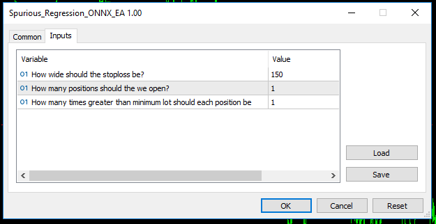
Fig 11: Our Expert Advisor.

And should automatically place stop losses and take profit levels for each trade it opens.

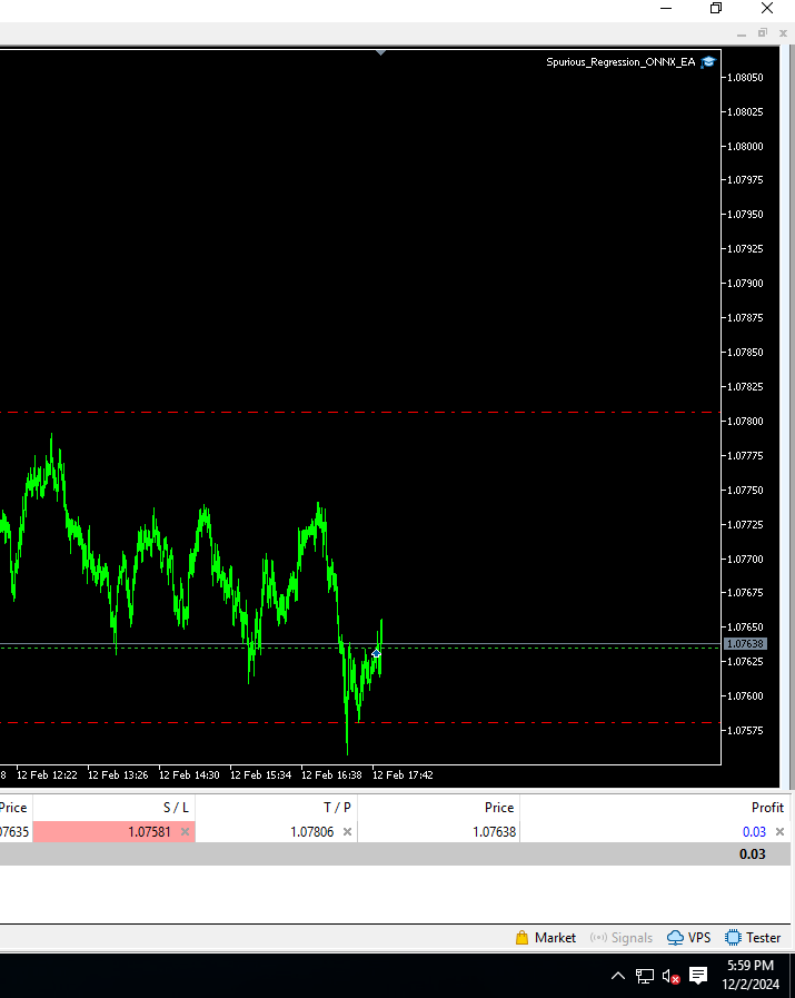
Fig 12: Our Expert Advisor in action.

Conclusion

In conclusion, spurious regressions pose a significant challenge when modelling time series data, often leading to misleading and unreliable results. Researchers and practitioners must exercise caution when interpreting regression outcomes, particularly when dealing with non-stationary time series data. To mitigate the risk of spurious regressions, employing appropriate statistical techniques, such as unit root tests, cointegration analysis, and utilizing stationary variables, is crucial. Furthermore, adopting advanced time series methods, such as error correction models, can enhance the robustness of regression analyses and contribute to more accurate and meaningful economic interpretations. Ultimately, a nuanced understanding of the underlying data properties and a rigorous application of statistical methods are essential for researchers seeking to produce reliable and valid regression results in the face of potential spurious relationships.