Creating Time Series Predictions using LSTM Neural Networks: Normalizing Price and Tokenizing Time

Introduction

I wanted to to explore the use of Neural Networks in developing a trading strategy so I delved into the topic by watching some Youtube Videos initially. Most were relatively confusing because they began at a very basic level such as how to program in Python: using strings, arrays, OOP and all the other basics. By the time the educator got to the actual crux of the course, Neural Networks and Machine Learning, you realized that they would simply be explaining how to use a particular library or a pre-trained model without actually explaining how they work. After much searching, I finally came across videos by Andrej Karpathy, which were fairly enlightening. Particularly, his video, Let's build GPT: from scratch, in code, spelled out allowed me to see how you can simple mathematical concepts, couple them with code, and bring human like intelligence to life just with a few hundred lines of code. The video sort of unlocked the world of neural networks for me in a relatively intuitive and practical way allowing me to experience their power first hand. Coupling some basic understanding from his channel, with assistance of 100s of ChatGPT queries to understand how they work, how to write them in Python, etc. I was able to come up a methodology to use Neural Networks in making predictions and building expert advisors. In this article I would like to not only document that journey but also display what I have learned and how a simple neural network like LSTM can be used to make market predictions.

LSTM Overview

When I started searching on the internet, I stumbled across some articles describing the use of LSTMs for time series predictions. Specifically, I came across a blog post by Christopher Olah, "Understanding LSTM Networks" on colah's blog. In his blog, Olah explains the structure and function of LSTMs, compares them to standard RNNs, and discusses various LSTM variants, such as those with peephole connections or Gated Recurrent Units (GRUs). Olah concludes by highlighting the significant impact of LSTMs on RNN applications and pointing towards future advancements like attention mechanisms.

In essence, traditional neural networks struggle with tasks requiring context from previous inputs due to their lack of memory. RNNs address this by having loops that allow information to persist, but they still face difficulties with long-term dependencies. For example, predicting the next word in a sentence where relevant context is many words back can be challenging for standard RNNs.  Long Short Term Memory (LSTM) networks are a type of recurrent neural network (RNN) designed to better handle long-term dependencies lacking in RNNs.

LSTMs solve this by using a more complex architecture, which includes a cell state and three types of gates (input, forget, and output) that regulate the flow of information. This design allows LSTMs to remember information for long periods, making them highly effective for tasks like language modeling, speech recognition, and image captioning. What I was interested in exploring was whether LSTMs can help predict price action today based on prior price action on days with similar price action due to their natural ability to remember information for longer periods of time. I came across another helpful article by Adrian Tam, astutely titled "LSTM for Time Series Prediction in PyTorch" that demystified math and the programming aspects for me with a practical example. I felt confident enough to take on the challenge of applying them in attempting to predict the future price action for any given currency pair.

Tokenization and Normalization Process

I devised a method to tokenize time within a given day and normalize price for a particular timeframe within the day to train the neural network; then, I found a way to use the trained neural network to make predictions; and finally, denormalize the prediction to get prediction of future price. This approach was inspired by the ChatGPT video I mentioned in my introduction. A similar strategy is used by LLMs to convert text strings into numerical and vector representations to train neural networks for language processing and response generation. In my case, for price, I wanted the data input into my neural network to be relative to the high or low of day on a rolling basis for the given day. The normalization and tokenization strategy that I used is given in the script below and summarized as follows: 

Time Tokenization

1. Conversion to Seconds: The script takes the time column (which is in datetime format) and converts it into a total number of seconds elapsed since the start of the day. This calculation includes hours, minutes, and seconds.

2. Normalization to Fraction of Day: The resulting number of seconds is then divided by the total number of seconds in a day (86400). This creates a time_token that represents time as a fraction of a day. For example: Noon would be 0.5 or 50% of the day completed.

Daily Rolling Price Normalization

1. Grouping by Date: The data is grouped by the date column to ensure normalization occurs independently for each trading day.

2. Rolling High/Low Calculation:

   • For each group (day), the script calculates the expanding maximum (rolling_high) and expanding minimum (rolling_low) of the high and low prices, respectively. This means that the rolling high/low only increases/decreases as new data comes in throughout the day.

3. Normalization:

   • The open , high , low , and close prices are normalized using the following formula: normalized_price = (price - rolling_low) / (rolling_high - rolling_low)
   • This scales each price to a range between 0 and 1 relative to the highest and lowest prices seen so far that day.
   • The normalization is done on a daily rolling basis, ensuring that price relationships within each day are captured while preventing the normalization from being affected by price movements across multiple days.
     

4. Handling NaNs: NaN values can occur at the beginning of a day before the rolling high/low is established. I considered 3 different approached to deal with them. The first approach was to drop them, the second approach was to forward fill them, and the third approach was to replace them with zeros. I decided to replace them with zeros after much testing and struggling with dropping them because ultimately my goal is to convert this process into an ONNX data processing pipeline that can be used directly with MQL5 to make predictions without replicating the code. I realized that ONNX is relatively rigid when it comes to input and output shapes and dropping NaNs values changes the shape of the output vector, which causes unexpected errors when using ONNX in MQL. I tried to use a forward filling method to replace the NaNs also, but this is a Pandas/NumPy method and does not conveniently translate to torch, which is the library I primarily used to convert my neural network model to ONNX. Finally, I decided to simply replace the NaNs with zeros, this seemed to work the best allowing me to side step the variable shapes issue, create a pipeline for the entire data processing and implement that in MQL through ONNX, thereby streamlining the entire process of getting a prediction within MQL. 

In summary, the normalization is done on a daily rolling basis, ensuring that price relationships within each day are captured while preventing the normalization from being affected by price movements across multiple days. Doing this puts prices on a similar scale, preventing the model from being biased towards features with larger magnitudes. It also helps adapt to the changing volatility within each day.

Code below helps visualize the process described above. If you download the zip file accompanying this article, you can find this code in the Folder Titled: "Visualizing the Normalization and Tokenization Process". The file is called: "visualizing.py"

import torch
import torch.nn as nn
import numpy as np
import pandas as pd
from sklearn.preprocessing import MinMaxScaler
import MetaTrader5 as mt5
import matplotlib.pyplot as plt
import joblib

# Connect to MetaTrader 5
if not mt5.initialize():
    print("Initialize failed")
    mt5.shutdown()

# Load market data
symbol = "EURUSD"
timeframe = mt5.TIMEFRAME_M15
rates = mt5.copy_rates_from_pos(symbol, timeframe, 0, 96)  # Note: 96 represents 1 day or 15*96= 1440 minutes of data (there are 1440 minutes in a day)
mt5.shutdown()

# Convert to DataFrame
data = pd.DataFrame(rates)
data['time'] = pd.to_datetime(data['time'], unit='s')
data.set_index('time', inplace=True)

# Tokenize time
data['time_token'] = (data.index.hour * 3600 + data.index.minute * 60 + data.index.second) / 86400

# Normalize prices on a rolling basis resetting at the start of each day
def normalize_daily_rolling(data):
    data['date'] = data.index.date
    data['rolling_high'] = data.groupby('date')['high'].transform(lambda x: x.expanding(min_periods=1).max())
    data['rolling_low'] = data.groupby('date')['low'].transform(lambda x: x.expanding(min_periods=1).min())

    data['norm_open'] = (data['open'] - data['rolling_low']) / (data['rolling_high'] - data['rolling_low'])
    data['norm_high'] = (data['high'] - data['rolling_low']) / (data['rolling_high'] - data['rolling_low'])
    data['norm_low'] = (data['low'] - data['rolling_low']) / (data['rolling_high'] - data['rolling_low'])
    data['norm_close'] = (data['close'] - data['rolling_low']) / (data['rolling_high'] - data['rolling_low'])

    # Replace NaNs with zeros
    data.fillna(0, inplace=True)
    return data

# Visualize the price before normalization
plt.figure(figsize=(15, 10))

plt.subplot(3, 1, 1)
data['close'].plot()
plt.title('Close Prices')
plt.xlabel('Time')
plt.ylabel('Price')

data = normalize_daily_rolling(data)

# Check for NaNs in the data
if data.isnull().values.any():
    print("Data contains NaNs")
    print(data.isnull().sum())

# Drop unnecessary columns
data = data[['time_token', 'norm_open', 'norm_high', 'norm_low', 'norm_close']]

# Visualize the normalized price
plt.subplot(3, 1, 2)
data['norm_close'].plot()
plt.title('Normalized Close Prices')
plt.xlabel('Time')
plt.ylabel('Normalized Price')

# Visualize Time After Tokenization
plt.subplot(3, 1, 3)
data['time_token'].plot()
plt.title('Time Token')
plt.xlabel('Time')
plt.ylabel('Time Token')

plt.tight_layout()
plt.show()

If you run the code above, you will see the approach I came up with in action. In the plot below from prices on 6/12/2024 entire day of trading overlapping into 6/13/2024. This was also a CPI and a Fed Meeting Day, two major red news events on the same day, which is relatively rare. You can see that the time token resets at the end of each day and increases linearly throughout the day. The price also resets, but this is a little harder to see in the plots. Any time a new high forms, the value of the normalized closed prices goes to 1. When a new low forms, the value of the normalized close prices goes to 0. 

Training and Validation Summary of Steps

The code below trains an LSTM (Long Short-Term Memory) model for predicting prices, specifically focusing on the EURUSD currency pair. User can change "EURUSD" to any other pair they desire to work with. 

Data Preparation

1. Retrieves Data: Connects to MetaTrader 5 platform to fetch historical price data (high, low, open, close) for EURUSD in 15-minute intervals. Again, you can pick your preferred timeframe 1 min, 5 min, 15 min etc. depending on your personal style.
2. Preprocesses Data:
   • Converts the data to a Pandas DataFrame, sets the timestamp as the index.
   • Creates a 'time_token' feature representing time as a fraction of the day.
   • Normalizes prices within each day based on rolling high/low on a continuous basis to account for daily fluctuations.
   • Handles missing values (NAN) by replacing them with zeros.
   • Drops unnecessary columns, such as, tick volumes, real volume, and spread.
3. Creates Sequences: Structures the data into sequences of 60 timesteps, where each sequence becomes an input (X) and the following closing price is the target (y).
4. Splits Data: Divides the sequences into training (80%) and testing (20%) sets.
5. Converts to Tensors: Transforms data into PyTorch tensors for model compatibility.

Model Definition and Training

1. Defines LSTM Model: Creates a class for the LSTM model with:
   • An LSTM layer that processes the sequence data.
   • A linear layer that produces the final prediction.
   • Internal state variables for the LSTM.
2. Sets Up Training:
   • Defines Mean Squared Error (MSE) as the loss function to be minimized.
   • Uses the Adam optimizer for adjusting model weights.
   • Sets a random seed for reproducibility.
3. Trains the Model:
   • Iterates over 100 epochs (full passes through the training data).
   • For each sequence in the training set:
     • Resets the LSTM's hidden state.
     • Passes the sequence through the model to get a prediction.
     • Calculates the MSE loss between the prediction and true value.
     • Performs backpropagation to update model weights.
   • Prints the loss every 10 epochs.
4. Saves Model: Preserves the trained model's parameters. File is saved as "lstm_model.pth" in the same folder as the one used to run the LSTM_model_training.py file. Also converts the model to ONNX format for use with MQL5 Directly. ONNX file is called "lstm_model.onnx". Note: that the shape of the vector required for prediction is seq_length, 1, input_size, which is 60, 1, 5 indicating that 60 prior bars of 15 minute data is required as 1 batch, with 5 values (time_token, norm_open, norm_high, norm_low, and norm_close) which all are between 0 and 1. We will use this later on in this article to create a data processing pipeline in ONNX for use with our model. 

Evaluation

1. Generates Predictions:
   • Switches the model to evaluation mode.
   • Iterates over sequences in the test set and generates predictions.
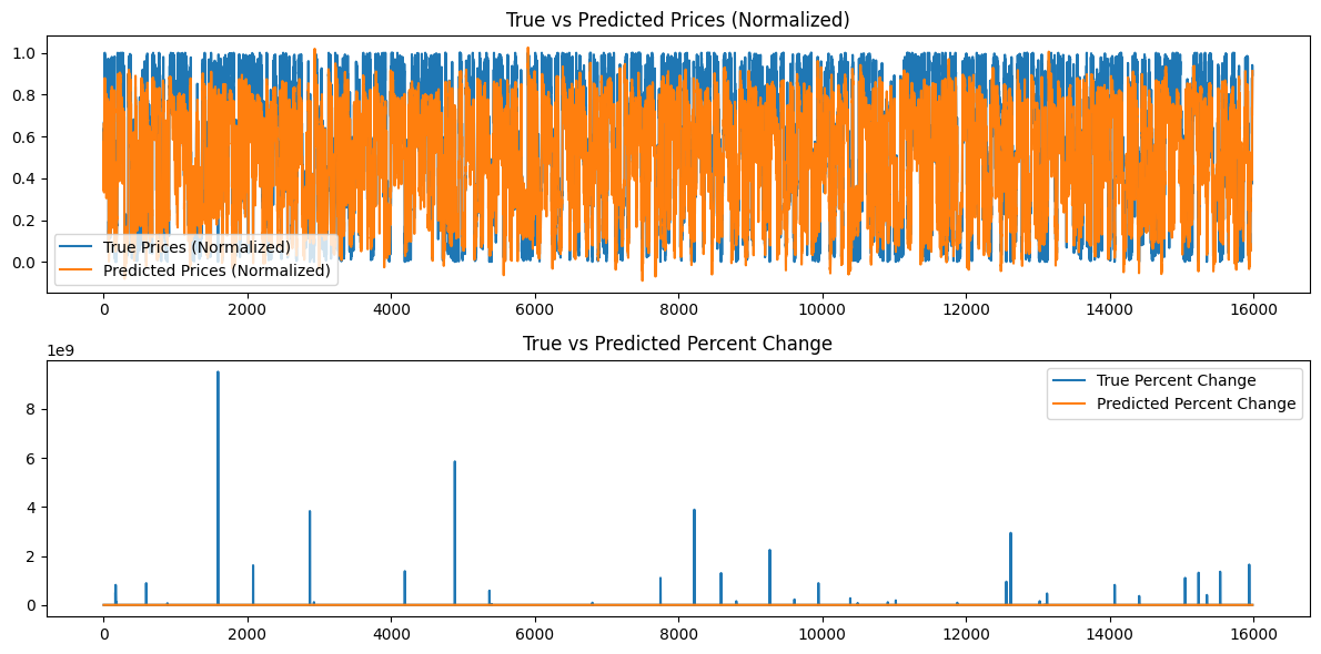
2. Visualizes Results:
• Plots the true normalized prices and predicted normalized prices.
• Calculates and plots the percent change in prices for both true and predicted values.

Model Parameter Selection: 

1. A majority of this code is written to focus on finding trends intraday. However, it can easily be adapted to other timeframes, such as weekly, monthly etc. The only issue for me was availability of data. Otherwise I could have expanded the code to include some of these other timeframes as well. 
2. I chose to work with the 15 minute timeframe because I could get approximately 80,000 bars of data to feed into my neural network. This is approximately 3 years of trading data (excluding weekends), which felt sufficient enough to build a decent LSTM neural network that attempts to predict intraday price action. 
3. The overall basis for the model is the following 5 parameters: time_token, norm_open, norm_high, norm_low, norm_close. Therefore the input_size = 5. There are three additional parameters I chose to ignore: tick volumes, real volumes, and spread. I excluded tick volumes because I couldn't find a trustworthy enough data source to ensure that they were reliable and trustworthy enough. I excluded real volumes for my broker doesn't have them available and they are always reported as zero. Lastly, I excluded spread because I fetched the data from a demo account, so they do not match live account broker spreads. 
4. Hidden Layers were chosen to be 100. This is an arbitrary value that I chose that seemed to work well. 
5. The value for output_size = 1 because the way this model is designed, we only care about the prediction for the next 15 minute bar. 
6. I chose a split of 80% for training vs. 20% for testing. This is also an arbitrary choice. Some people prefer 50:50 split, others prefer 70:30 split. I just wasn't too sure, so I just decided to go with 80:20 for my split. 
7. I chose a seed value of 42. My main goal was to have some reproducibility in results from trial to trail. Therefore I specified the seed value so I could compare the results on an even basis in case I decide to play with any parameters in the future. 
8. I chose a learning rate value of 0.001. This is again an arbitrary choice. User is free to set his or her learning rate as he or she sees fit. 
9. I selected the sequence length (seq_length) of 60. Basically this is how many bars of "context" the LSTM model needs to make the prediction about the next bar. This was an arbitrary choice as well. 60 * 15 mins = 900 minutes or 15 hours. That's a lot of time to get context to be able to predict one 15 minute bar and may be a little excessive. I don't have a great justification for picking this value; however, the model is flexible, and users are free to change these values as they see fit. 
10. Training Time: 100 epochs was chosen because the model with 80,000 bars would take approximately 8 hours to run on my computer. I used CPU for training. As I wrote this article, I made several refinements to my code and had to re-run the model multiple times. So 8 hours training time was I could afford to run for the model.

Here is the full code that I came up with. It can be found in the root of the attached zipped folder and it is called LSTM_model_training.py. 

import torch
import torch.nn as nn
import numpy as np
import pandas as pd
import MetaTrader5 as mt5
import matplotlib.pyplot as plt
import torch.onnx
import torch.nn.functional as F

# Connect to MetaTrader 5
if not mt5.initialize():
    print("Initialize failed")
    mt5.shutdown()

# Load market data
symbol = "EURUSD"
timeframe = mt5.TIMEFRAME_M15
rates = mt5.copy_rates_from_pos(symbol, timeframe, 0, 80000)
mt5.shutdown()

# Convert to DataFrame
data = pd.DataFrame(rates)
data['time'] = pd.to_datetime(data['time'], unit='s')
data.set_index('time', inplace=True)

# Tokenize time
data['time_token'] = (data.index.hour * 3600 + data.index.minute * 60 + data.index.second) / 86400

# Normalize prices on a rolling basis resetting at the start of each day
def normalize_daily_rolling(data):
    data['date'] = data.index.date
    data['rolling_high'] = data.groupby('date')['high'].transform(lambda x: x.expanding(min_periods=1).max())
    data['rolling_low'] = data.groupby('date')['low'].transform(lambda x: x.expanding(min_periods=1).min())

    data['norm_open'] = (data['open'] - data['rolling_low']) / (data['rolling_high'] - data['rolling_low'])
    data['norm_high'] = (data['high'] - data['rolling_low']) / (data['rolling_high'] - data['rolling_low'])
    data['norm_low'] = (data['low'] - data['rolling_low']) / (data['rolling_high'] - data['rolling_low'])
    data['norm_close'] = (data['close'] - data['rolling_low']) / (data['rolling_high'] - data['rolling_low'])

    # Replace NaNs with zeros
    data.fillna(0, inplace=True)
    return data

data = normalize_daily_rolling(data)

# Check for NaNs in the data
if data.isnull().values.any():
    print("Data contains NaNs")
    print(data.isnull().sum())

# Drop unnecessary columns
data = data[['time_token', 'norm_open', 'norm_high', 'norm_low', 'norm_close']]

# Create sequences
def create_sequences(data, seq_length):
    xs, ys = [], []
    for i in range(len(data) - seq_length):
        x = data.iloc[i:(i + seq_length)].values
        y = data.iloc[i + seq_length]['norm_close']
        xs.append(x)
        ys.append(y)
    return np.array(xs), np.array(ys)

seq_length = 60
X, y = create_sequences(data, seq_length)

# Split data
split = int(len(X) * 0.8)
X_train, X_test = X[:split], X[split:]
y_train, y_test = y[:split], y[split:]

# Convert to tensors
X_train = torch.tensor(X_train, dtype=torch.float32)
y_train = torch.tensor(y_train, dtype=torch.float32)
X_test = torch.tensor(X_test, dtype=torch.float32)
y_test = torch.tensor(y_test, dtype=torch.float32)

# Set the seed for reproducibility
seed_value = 42
torch.manual_seed(seed_value)

# Define LSTM model class
class LSTMModel(nn.Module):
    def __init__(self, input_size, hidden_layer_size, output_size):
        super(LSTMModel, self).__init__()
        self.hidden_layer_size = hidden_layer_size
        self.lstm = nn.LSTM(input_size, hidden_layer_size)
        self.linear = nn.Linear(hidden_layer_size, output_size)

    def forward(self, input_seq):
        h0 = torch.zeros(1, input_seq.size(1), self.hidden_layer_size).to(input_seq.device)
        c0 = torch.zeros(1, input_seq.size(1), self.hidden_layer_size).to(input_seq.device)
        lstm_out, _ = self.lstm(input_seq, (h0, c0))
        predictions = self.linear(lstm_out.view(input_seq.size(0), -1))
        return predictions[-1]

print(f"Seed value used: {seed_value}")

input_size = 5  # time_token, norm_open, norm_high, norm_low, norm_close
hidden_layer_size = 100
output_size = 1

model = LSTMModel(input_size, hidden_layer_size, output_size)
#model = torch.compile(model)
loss_function = nn.MSELoss()
optimizer = torch.optim.Adam(model.parameters(), lr=0.001)

# Training
epochs = 100
for epoch in range(epochs + 1):
    for seq, labels in zip(X_train, y_train):
        optimizer.zero_grad()
        y_pred = model(seq.unsqueeze(1))

        # Ensure both are tensors of shape [1]
        y_pred = y_pred.view(-1)
        labels = labels.view(-1)

        single_loss = loss_function(y_pred, labels)
        
        # Print intermediate values to debug NaN loss
        if torch.isnan(single_loss):
            print(f'Epoch {epoch} NaN loss detected')
            print('Sequence:', seq)
            print('Prediction:', y_pred)
            print('Label:', labels)

        single_loss.backward()
        optimizer.step()

    if epoch % 10 == 0 or epoch == epochs:  # Include the final epoch
        print(f'Epoch {epoch} loss: {single_loss.item()}')

# Save the model's state dictionary
torch.save(model.state_dict(), 'lstm_model.pth')

# Convert the model to ONNX format
model.eval()
dummy_input = torch.randn(seq_length, 1, input_size, dtype=torch.float32)
onnx_model_path = "lstm_model.onnx"
torch.onnx.export(model, 
                  dummy_input, 
                  onnx_model_path, 
                  input_names=['input'], 
                  output_names=['output'],
                  dynamic_axes={'input': {0: 'sequence'}, 'output': {0: 'sequence'}},
                  opset_version=11)

print(f"Model has been converted to ONNX format and saved to {onnx_model_path}")

# Predictions
model.eval()
predictions = []
for seq in X_test:
    with torch.no_grad():
        predictions.append(model(seq.unsqueeze(1)).item())

# Evaluate the model
plt.plot(y_test.numpy(), label='True Prices (Normalized)')
plt.plot(predictions, label='Predicted Prices (Normalized)')
plt.legend()
plt.show()

# Calculate percent changes with a small value added to the denominator to prevent divide by zero error
true_prices = y_test.numpy()
predicted_prices = np.array(predictions)

true_pct_change = np.diff(true_prices) / (true_prices[:-1] + 1e-10)
predicted_pct_change = np.diff(predicted_prices) / (predicted_prices[:-1] + 1e-10)

# Plot the true and predicted prices
plt.figure(figsize=(12, 6))
plt.subplot(2, 1, 1)
plt.plot(true_prices, label='True Prices (Normalized)')
plt.plot(predicted_prices, label='Predicted Prices (Normalized)')
plt.legend()
plt.title('True vs Predicted Prices (Normalized)')

# Plot the percent change
plt.subplot(2, 1, 2)
plt.plot(true_pct_change, label='True Percent Change')
plt.plot(predicted_pct_change, label='Predicted Percent Change')
plt.legend()
plt.title('True vs Predicted Percent Change')

plt.tight_layout()
plt.show()

Model Evaluation Results

The training time was approximately 8 hours for 100 epochs. The model was not trained using a GPU. I used my own PC, which is a 4-year old gaming machine with the following specs: AMD Ryzen 5 4600H with Radeon Graphics 3.00 GHz and installed RAM of 64 GB. 

The Seed Value and Mean Squared Error Loss for Every 10 Epochs are printed on the console

• Seed value used: 42
• Epoch 0 loss: 0.01435865368694067
• Epoch 10 loss: 0.014593781903386116
• Epoch 20 loss: 0.02026239037513733
• Epoch 30 loss: 0.017134636640548706
• Epoch 40 loss: 0.017405137419700623
• Epoch 50 loss: 0.004391830414533615
• Epoch 60 loss: 0.0210900716483593
• Epoch 70 loss: 0.008576949127018452
• Epoch 80 loss: 0.019675739109516144
• Epoch 90 loss: 0.008747504092752934
• Epoch 100 loss: 0.033280737698078156

At the end of the training, I also received a warning shown below. The warning suggests specifying the model a different way. I fiddled around with trying to fix it. But due to the extensive training time, I decided to ignore the warning because the sequences in our batch will not have different lengths. 

Additionally the following graphs are generated: 

Analysis of Model Results

The epoch losses for a seed value of 42 seem to decrease erratically. Since they are not monotonic, perhaps the model could benefit from further training. Alternatively, the user may consider providing a different seed value or using a random seed value automatically generated by the Torch library in Python and printing out this value using the torch.seed() command. Additionally, the model performance may also improve if the amount of available data is increased; however by doing so, the user may experience additional computational costs associated with longer training times and greater hardware memory requirements.

The graphs generated attempt to summarize over 16000 bars of 15 minute data. Therefore, the graphing system I used is not very effective because most of the data becomes squished and hard to asses. These graphs are more "global" representations of the overall training that took place. As is they add no value. I have included them for reference because I trained the model with smaller datasets as well, and they were helpful; however for 80,000 bars, they are not very useful. We will address this problem in the next section when we will try to make predictions based on our generated model and the data will be a "local" representation, that is, day to day price action. We will create a continuous prediction based on our model in the next section by utilizing our sequence length of 60 and adding 100 more bars (160 total bars of 15 minute data) to and continuously make a prediction from bar 100 to 0 and represent that on a graph that will perhaps be more enlightening. 

Making Predictions Using The Trained Model (Using Python)

To create a prediction script, we would ideally use the last 60 values from the EURUSD data on a 15-minute timeframe to make a prediction using the saved LSTM model. However, I felt it would be better to get a rolling prediction along with a graph in python so I could quickly validate the model before using this. Here are the key features of the prediction script for Python use-case. A Summary of the script is given below: 

• LSTM Model Definition: The script defines the structure of the LSTM model. The model consists of an LSTM layer followed by a linear layer. This is identical to what we used for training the model in the training script above. 

• Data Preparation:

  • It connects to MetaTrader 5 to retrieve the latest 160 bars (15-minute intervals) of EURUSD data. Note even though we only need 60 bars of 15 minute data to make a prediction, we will pull 160 bars to predict and compare the last 100 predictions. This will give us some sense of the underlying trend of predicted vs. actual. 
  • The data is converted to a pandas DataFrame and normalized using the same rolling normalization technique used during training.
  • Time tokenization is applied to convert time into a numerical representation.

• Model Loading:

  • The trained LSTM model (from 'lstm_model.pth') is loaded. This is the model that we trained during the training phase. 

• Evaluation:

  • The script iterates through the last 100 steps of the data.
  • For each step, it takes the 60 previous bars as input and uses the model to predict the normalized closing price.
  • True and predicted prices are stored for comparison.

• Next Prediction:

  • It makes a prediction for the next step using the most recent 60 bars.
  • Calculates the percent change for this prediction.
  • Shows the prediction as a red dot on the chart. 

• Visualization:

  • Two plots are generated:
    • True vs. Predicted Prices (Normalized) with the next prediction highlighted.
    • True vs. Predicted Price Percent Change with the next prediction highlighted.
  • Y-axes are capped to 100% for better visualization.  

The code below can be found in the file "LSTM_model_prediction.py", which is located in the root of the LSTM_Files.zip attached to this article. 

import torch
import torch.nn as nn
import numpy as np
import pandas as pd
import MetaTrader5 as mt5
import matplotlib.pyplot as plt

# Define LSTM model class (same as during training)
class LSTMModel(nn.Module):
    def __init__(self, input_size, hidden_layer_size, output_size):
        super(LSTMModel, self).__init__()
        self.hidden_layer_size = hidden_layer_size
        self.lstm = nn.LSTM(input_size, hidden_layer_size)
        self.linear = nn.Linear(hidden_layer_size, output_size)
        self.hidden_cell = (torch.zeros(1, 1, self.hidden_layer_size),
                            torch.zeros(1, 1, self.hidden_layer_size))

    def forward(self, input_seq):
        lstm_out, self.hidden_cell = self.lstm(input_seq.view(len(input_seq), 1, -1), self.hidden_cell)
        predictions = self.linear(lstm_out.view(len(input_seq), -1))
        return predictions[-1]

# Normalize prices on a rolling basis resetting at the start of each day
def normalize_daily_rolling(data):
    data['date'] = data.index.date
    data['rolling_high'] = data.groupby('date')['high'].transform(lambda x: x.expanding(min_periods=1).max())
    data['rolling_low'] = data.groupby('date')['low'].transform(lambda x: x.expanding(min_periods=1).min())

    data['norm_open'] = (data['open'] - data['rolling_low']) / (data['rolling_high'] - data['rolling_low'])
    data['norm_high'] = (data['high'] - data['rolling_low']) / (data['rolling_high'] - data['rolling_low'])
    data['norm_low'] = (data['low'] - data['rolling_low']) / (data['rolling_high'] - data['rolling_low'])
    data['norm_close'] = (data['close'] - data['rolling_low']) / (data['rolling_high'] - data['rolling_low'])

    # Replace NaNs with zeros
    data.fillna(0, inplace=True)
    return data[['norm_open', 'norm_high', 'norm_low', 'norm_close']]

# Load the saved model
input_size = 5  # time_token, norm_open, norm_high, norm_low, norm_close
hidden_layer_size = 100
output_size = 1

model = LSTMModel(input_size, hidden_layer_size, output_size)
model.load_state_dict(torch.load('lstm_model.pth'))
model.eval()

# Connect to MetaTrader 5
if not mt5.initialize():
    print("Initialize failed")
    mt5.shutdown()

# Load the latest 160 bars of market data
symbol = "EURUSD"
timeframe = mt5.TIMEFRAME_M15
bars = 160  # 60 for sequence length + 100 for evaluation steps
rates = mt5.copy_rates_from_pos(symbol, timeframe, 0, bars)
mt5.shutdown()

# Convert to DataFrame
data = pd.DataFrame(rates)
data['time'] = pd.to_datetime(data['time'], unit='s')
data.set_index('time', inplace=True)

# Normalize the new data
data[['norm_open', 'norm_high', 'norm_low', 'norm_close']] = normalize_daily_rolling(data)

# Tokenize time
data['time_token'] = (data.index.hour * 3600 + data.index.minute * 60 + data.index.second) / 86400

# Drop unnecessary columns
data = data[['time_token', 'norm_open', 'norm_high', 'norm_low', 'norm_close']]

# Fetch the last 100 sequences for evaluation
seq_length = 60
evaluation_steps = 100

# Initialize lists for storing evaluation results
all_true_prices = []
all_predicted_prices = []

model.eval()

for step in range(evaluation_steps, 0, -1):
    # Get the sequence ending at 'step'
    seq = data.values[-step-seq_length:-step]
    seq = torch.tensor(seq, dtype=torch.float32)

    # Make prediction
    with torch.no_grad():
        model.hidden_cell = (torch.zeros(1, 1, model.hidden_layer_size),
                             torch.zeros(1, 1, model.hidden_layer_size))
        prediction = model(seq).item()
    
    all_true_prices.append(data['norm_close'].values[-step])
    all_predicted_prices.append(prediction)

# Calculate percent changes and convert to percentages
true_pct_change = (np.diff(all_true_prices) / np.array(all_true_prices[:-1])) * 100
predicted_pct_change = (np.diff(all_predicted_prices) / np.array(all_predicted_prices[:-1])) * 100

# Make next prediction
next_seq = data.values[-seq_length:]
next_seq = torch.tensor(next_seq, dtype=torch.float32)

with torch.no_grad():
    model.hidden_cell = (torch.zeros(1, 1, model.hidden_layer_size),
                         torch.zeros(1, 1, model.hidden_layer_size))
    next_prediction = model(next_seq).item()

# Calculate percent change for the next prediction
next_true_price = data['norm_close'].values[-1]
next_price_pct_change = ((next_prediction - all_predicted_prices[-1]) / all_predicted_prices[-1]) * 100

print(f"Next predicted close price (normalized): {next_prediction}")
print(f"Percent change for the next prediction based on normalized price: {next_price_pct_change:.5f}%")
print("All Predicted Prices: ", all_predicted_prices)

# Plot the evaluation results with capped y-axis
plt.figure(figsize=(12, 8))

plt.subplot(2, 1, 1)
plt.plot(all_true_prices, label='True Prices (Normalized)')
plt.plot(all_predicted_prices, label='Predicted Prices (Normalized)')
plt.scatter(len(all_true_prices), next_prediction, color='red', label='Next Prediction')
plt.legend()
plt.title('True vs Predicted Prices (Normalized, Last 100 Steps)')
plt.ylim(min(min(all_true_prices), min(all_predicted_prices))-0.1, max(max(all_true_prices), max(all_predicted_prices))+0.1)

plt.subplot(2, 1, 2)
plt.plot(true_pct_change, label='True Percent Change')
plt.plot(predicted_pct_change, label='Predicted Percent Change')
plt.scatter(len(true_pct_change), next_price_pct_change, color='red', label='Next Prediction')
plt.legend()
plt.title('True vs Predicted Price Percent Change (Last 100 Steps)')
plt.ylabel('Percent Change (%)')
plt.ylim(-100, 100)  # Cap the y-axis at -100% to 100%

plt.tight_layout()
plt.show()

Below is the output that we get on the console and the graphs that we obtain. This prediction was generated right at the start of the day on 6/14/2024 (Approximately Broker Time 00:45 UTC + 3)

Console Output: 

Next predicted close price (normalized): 0.9003118872642517

Percent change for the next prediction based on normalized price: 73.64274%

All Predicted Prices: [0.6229779124259949, 0.6659790277481079, 0.6223553419113159, 0.5994003415107727, 0.565409243106842, 0.5767043232917786, 0.5080181360244751, 0.5245669484138489, 0.6399291753768921, 0.5184902548789978, 0.6269711256027222, 0.6532717943191528, 0.7470211386680603, 0.6783792972564697, 0.6942530870437622, 0.6399927139282227, 0.5649009943008423, 0.6392825841903687, 0.6454082727432251, 0.4829435348510742, 0.5231367349624634, 0.17141318321228027, 0.3651347756385803, 0.2568517327308655, 0.41483253240585327, 0.43905267119407654, 0.40459558367729187, 0.25486069917678833, 0.3488359749317169, 0.41225481033325195, 0.13895493745803833, 0.21675345301628113, 0.04991495609283447, 0.28392884135246277, 0.17570143938064575, 0.34913408756256104, 0.17591500282287598, 0.33855849504470825, 0.43142321705818176, 0.5618296265602112, 0.0774659514427185, 0.13539350032806396, 0.4843936562538147, 0.5048894882202148, 0.8364744186401367, 0.782444417476654, 0.7968958616256714, 0.7907949686050415, 0.5655181407928467, 0.6196668744087219, 0.7133172750473022, 0.5095566511154175, 0.3565239906311035, 0.2686333656311035, 0.3386841118335724, 0.5644893646240234, 0.23622554540634155, 0.3433009088039398, 0.3493557274341583, 0.2939424216747284, 0.08992069959640503, 0.33946871757507324, 0.20876094698905945, 0.4227801263332367, 0.4044940173625946, 0.654332160949707, 0.49300187826156616, 0.6266812086105347, 0.807404637336731, 0.5183461904525757, 0.46170246601104736, 0.24424996972084045, 0.3224128782749176, 0.5156376957893372, 0.06813174486160278, 0.1865384578704834, 0.15443122386932373, 0.300825834274292, 0.28375834226608276, 0.4036571979522705, 0.015333771705627441, 0.09899216890335083, 0.16346102952957153, 0.27330827713012695, 0.2869266867637634, 0.21237093210220337, 0.35913240909576416, 0.4736405313014984, 0.3459511995315552, 0.47014304995536804, 0.3305799663066864, 0.47306257486343384, 0.4134630858898163, 0.4199170768260956, 0.5666837692260742, 0.46681761741638184, 0.35662856698036194, 0.3547590374946594, 0.5447400808334351, 0.5184851884841919]

Analysis of Prediction Results

The console output is  0.9003118872642517, which indicates that the next price move is likely going to be 0.9 of the current daily range, which is approximately between 1.07402 and 1.07336 or ~8 pips. This may not be enough of a price change, which is understandable because at the time of this writing, we had only had ~45 minutes of trading on 6/14/2024. However, the model does predict that the price will close near the upper end of the current daily range. 

The next line is:  Percent change for the next prediction based on normalized price: 73.64274%. This suggests that the next price change is likely to be about +74% above the previous price, which when put in context if 8 pips daily range, may not offer adequate number of pips to place a trade. 

Instead of working with numbers and fractions, the user may consider adding a line that takes the daily (high - low) and multiplies it by the normalized predicted close price, to get an actual value of pips they can anticipate. We will not only do this when we convert our script to MQL, but we will also get an exact price prediction.

As you can see in the output above, a list of 100 predictions are also printed to the console. We can use these values for validation, especially when we transition to MQL5 and start using the script there. 

Lastly we also get a graph from the Matplotlib library in Python gives us a set of last 100 predictions, graphs them, and compares them to the actual changes in the closing prices on a normalized basis (0 to 1 scale). The red dot shows the next most likely price on a normalized basis giving us an indication of the possible next price direction. Based on this particular day of data, our prediction seems to be lagging behind the market, indicating that the predicted results may not be well aligned with the actual price action for the day. On such a day, a discretionary trader or user should consider staying on the sidelines and not trading because the model does not make predictions accurately. Note this does not necessarily mean that the model predictions are incorrect over the entire dataset, therefore retraining may not be necessary either. 

Transitioning from Python to ONNX and Using The Trained Model with MQL5 Directly

Creating a Data Processing Pipeline 

The idea for creating a data processing pipeline for me was to not replicate the normalization and tokenization code that I created in Python. I didn't want to rewrite that code in MQL. So I decided to convert the script into a data pipeline, convert it to ONNX, and use the ONNX directly for data processing in MQL. It took me several days to figure out the code to do this due to my lack of prior experience with creating data processing pipelines. The reason I struggled is because Python is relatively flexible when it comes to data types. But when converting to ONNX, you have to be a lot more rigid, and specific. I encountered numerous errors along the way. Finally, when I figured it out I was very happy and I am happy to share the script below. Here is a quick summary of how the script works: 

As we noted in our discussion earlier, the preprocessing consists of two crucial steps:

1. Time Tokenization: It transforms the raw time of day (e.g., 3:45 PM) into a fractional value between 0 and 1, representing the portion of the 24-hour day that has elapsed.

2. Daily Rolling Normalization: This process standardizes the price data (open, high, low, close) on a daily basis. It calculates the rolling minimum and maximum prices within each day and normalizes the prices relative to these values. This normalization helps with model training by ensuring the price data has a consistent scale.

Components:

• TimeTokenizer (Custom Transformer): This class handles the time tokenization. It extracts the time column from the input tensor, converts it into a fractional representation of the day, and then combines it back with the other price data.

• DailyRollingNormalizer (Custom Transformer): This class performs the daily rolling normalization. It iterates through the price data, keeping track of the rolling maximum and minimum for each day. The prices are then normalized using these dynamic values. It also includes a step to replace any potential NaN values that might arise during calculation.

• ReplaceNaNs (Custom Transformer): Replaces all NaN values from the calculation with zeros.

• Pipeline (nn.Sequential): This combines the above three custom transformers into a sequential workflow. The input data passes through the TimeTokenizer, then the DailyRollingNormalizer, and lastly the ReplaceNaNs in that order.

• MetaTrader5 Connection: The script establishes a connection to MetaTrader 5 to retrieve historical EUR/USD price data.

Execution:

1. Data Loading: The script fetches 160 bars (price data points) from MetaTrader 5 for the EURUSD pair on the 15 minute timeframe.

2. Data Conversion: The raw data is converted into a PyTorch tensor for further processing.

3. Pipeline Processing: The tensor is passed through the defined pipeline , applying the time tokenization and daily rolling normalization steps.

4. ONNX Export: The final preprocessed data is printed to the console to show before and after results. Additionally, the entire preprocessing pipeline is exported to an ONNX file. ONNX is an open format that allows machine learning models to be easily transferred between different frameworks and environments, ensuring broader compatibility for model deployment and usage.

Key Points:

• Modularity: The use of custom transformers makes the code modular and reusable. Each transformer encapsulates a specific preprocessing step.
• PyTorch: The script relies on PyTorch, a popular deep learning framework, for tensor operations and model management.
• ONNX Export: Exporting to ONNX ensures the preprocessing steps can be seamlessly integrated with different platforms or tools where the trained model is deployed.

The code below can be found inside the folder "ONNX Data Pipeline" in the file called "LSTM Data Pipeline.py". These are located in the LSTM_Files.zip attached as part of the article. 

import torch
import torch.nn as nn
import pandas as pd
import MetaTrader5 as mt5

# Custom Transformer for tokenizing time
class TimeTokenizer(nn.Module):
    def forward(self, X):
        time_column = X[:, 0]  # Assuming 'time' is the first column
        time_token = (time_column % 86400) / 86400
        time_token = time_token.unsqueeze(1)  # Add a dimension to match the input shape
        return torch.cat((time_token, X[:, 1:]), dim=1)  # Concatenate the time token with the rest of the input

# Custom Transformer for daily rolling normalization
class DailyRollingNormalizer(nn.Module):
    def forward(self, X):
        time_tokens = X[:, 0]  # Assuming 'time_token' is the first column
        price_columns = X[:, 1:]  # Assuming 'open', 'high', 'low', 'close' are the remaining columns

        normalized_price_columns = torch.zeros_like(price_columns)
        rolling_max = price_columns.clone()
        rolling_min = price_columns.clone()

        for i in range(1, price_columns.shape[0]):
            reset_mask = (time_tokens[i] < time_tokens[i-1]).float()
            rolling_max[i] = reset_mask * price_columns[i] + (1 - reset_mask) * torch.maximum(rolling_max[i-1], price_columns[i])
            rolling_min[i] = reset_mask * price_columns[i] + (1 - reset_mask) * torch.minimum(rolling_min[i-1], price_columns[i])
            denominator = rolling_max[i] - rolling_min[i]
            normalized_price_columns[i] = (price_columns[i] - rolling_min[i]) / denominator

        time_tokens = time_tokens.unsqueeze(1)  # Assuming 'time_token' is the first column
        return torch.cat((time_tokens, normalized_price_columns), dim=1)

class ReplaceNaNs(nn.Module):
    def forward(self, X):
        X[torch.isnan(X)] = 0
        X[X != X] = 0  # replace negative NaNs with 0
        return X

# Connect to MetaTrader 5
if not mt5.initialize():
    print("Initialize failed")
    mt5.shutdown()

# Load market data (reduced sample size for demonstration)
symbol = "EURUSD"
timeframe = mt5.TIMEFRAME_M15
rates = mt5.copy_rates_from_pos(symbol, timeframe, 0, 160) #intialize with maximum number of bars allowed by your broker
mt5.shutdown()

# Convert to DataFrame and keep only 'time', 'open', 'high', 'low', 'close' columns
data = pd.DataFrame(rates)[['time', 'open', 'high', 'low', 'close']]

# Convert the DataFrame to a PyTorch tensor
data_tensor = torch.tensor(data.values, dtype=torch.float32)

# Create the updated pipeline
pipeline = nn.Sequential(
    TimeTokenizer(),
    DailyRollingNormalizer(),
    ReplaceNaNs()
)

# Print the data before processing
print('Data Before Processing\n', data[:100])

# Process the data
processed_data = pipeline(data_tensor)

print('Data After Processing\n', processed_data[:100])

# Export the pipeline to ONNX format
dummy_input = torch.randn(len(data), len(data.columns))
torch.onnx.export(pipeline, dummy_input, "data_processing_pipeline.onnx", input_names=["input"], output_names=["output"])

The output from the code gives the data before processing and after processing printed on the console. I won't reproduce that output because it's not important, but the user can consider running the script to see the output themselves. Additionally, the output creates a file: data_processing_pipeline.onnx. To validate the shape used by this ONNX model, I created a script as follows: 

This script can be found in the ONNX Data Pipeline Folder and is called "shape_check.py". These files are located in the LSTM_Files.zip attached to this article. 

import onnx

model = onnx.load("data_processing_pipeline.onnx")
onnx.checker.check_model(model)

for input in model.graph.input:
    print(f'Input name: {input.name}')
    print(f'Input type: {input.type}')
    for dim in input.type.tensor_type.shape.dim:
        print(dim.dim_value)

This gives the following result: 

• 160
• 5

Therefore the shape required by our model is 160 - 15 minute bars, and 5 value (time value as UNIX Integer, Open, High, Low, Close). After processing the data, the result will be the normalized data as time_token, norm_open, norm_high, norm_low, and norm_close. 

To test the data processing in MQL, I also came up with a specific script, which is called "LSTM Data Pipeline.mq5", located in the root folder of the attached zip file to validate that the data is being transformed the way I originally intended. This script can be found below. The key features are summarized as follows: 

• Initialization (OnInit):

  • Loads the ONNX model from the binary data ("data_processing_pipeline.onnx") embedded as a resource. Note that the ONNX model is stored inside a folder called "LSTM", which is a subfolder within the "Experts" folder as shown below.
  • Then we configure the model input and output shapes based on our ONNX code. So the "LSTM Data Pipeline Test.ex5" should be stored inside the Experts folder because we are using the following path. If you decide to store the file in some other manner, please update this line to ensure that the code works appropriately. 

  • #resource "\\LSTM\\data_processing_pipeline.onnx" as uchar ExtModel[]

    
    

• Tick Data Handling (OnTick):

  • This function is triggered on every price tick update.
  • It waits until the next bar (15-minute candle in this case) forms.
  • Calls the ProcessData function to handle data processing and prediction.

• Data Processing (ProcessData):

  • Fetches the latest SAMPLE_SIZE (160 in this case) bars of EURUSD M15 data. 
  • Extracts time, open, high, low, and close prices from the fetched data.
  • Normalizes the time component to represent a fraction of a day (between 0 and 1).
  • Prepares the input data for the ONNX model as a one-dimensional vector.
  • Executes the ONNX model ( OnnxRun ) with the prepared input vector.
  • Receives the processed output from the model.
  • Prints the processed data, which includes the time token and normalized prices.

//+------------------------------------------------------------------+
//|                                                  ONNX Test       |
//|                                                   Copyright 2023 |
//|                                               Your Name Here     |
//+------------------------------------------------------------------+
#property copyright   "Copyright 2023, Your Name Here"
#property link        "https://www.mql5.com"
#property version     "1.00"

static vectorf ExtOutputData(1);
vectorf output_data(1);

#include <Trade\Trade.mqh>
CTrade trade;

#resource "\\LSTM\\data_processing_pipeline.onnx" as uchar ExtModel[]

#define SAMPLE_SIZE 160  // Adjusted to match the model's expected input size

long     ExtHandle=INVALID_HANDLE;
datetime ExtNextBar=0;

// Expert Advisor initialization
int OnInit()
{
   // Load the ONNX model
   ExtHandle = OnnxCreateFromBuffer(ExtModel, ONNX_DEFAULT);
   if (ExtHandle == INVALID_HANDLE)
   {
      Print("Error creating model OnnxCreateFromBuffer ", GetLastError());
      return(INIT_FAILED);
   }

   // Set input shape




   const long input_shape[] = {SAMPLE_SIZE, 5};  // Adjust based on your model's input dimensions
   if (!OnnxSetInputShape(ExtHandle, ONNX_DEFAULT, input_shape))
   {
      Print("Error setting the input shape OnnxSetInputShape ", GetLastError());
      return(INIT_FAILED);
   }

   // Set output shape
   const long output_shape[] = {SAMPLE_SIZE, 5};  // Adjust based on your model's output dimensions
   if (!OnnxSetOutputShape(ExtHandle, 0, output_shape))
   {
      Print("Error setting the output shape OnnxSetOutputShape ", GetLastError());
      return(INIT_FAILED);
   }

   return(INIT_SUCCEEDED);
}

// Expert Advisor deinitialization
void OnDeinit(const int reason)
{
   if (ExtHandle != INVALID_HANDLE)
   {
      OnnxRelease(ExtHandle);
      ExtHandle = INVALID_HANDLE;
   }
}

// Process the tick function
void OnTick()
{
   if (TimeCurrent() < ExtNextBar)
      return;

   ExtNextBar = TimeCurrent();
   ExtNextBar -= ExtNextBar % PeriodSeconds();
   ExtNextBar += PeriodSeconds();

   // Fetch new data and run the ONNX model
   if (!ProcessData())
   {
      Print("Error processing data");
      return;
   }
}

// Function to process data using the ONNX model
bool ProcessData()
{
   MqlRates rates[SAMPLE_SIZE];
   int copied = CopyRates(_Symbol, PERIOD_M15, 1, SAMPLE_SIZE, rates);
   if (copied != SAMPLE_SIZE)
   {
      Print("Failed to copy the expected number of rates. Expected: ", SAMPLE_SIZE, ", Copied: ", copied);
      return false;
   }
   else if(copied == SAMPLE_SIZE)
   {
      Print("Successfully copied the expected number of rates. Expected: ", SAMPLE_SIZE, ", Copied: ", copied);
   }

   double min_time = rates[0].time;
   double max_time = rates[0].time;
   for (int i = 1; i < copied; i++)
   {
      if (rates[i].time < min_time)
         min_time = rates[i].time;
      if (rates[i].time > max_time)
         max_time = rates[i].time;
   }

   float input_data[SAMPLE_SIZE * 5];
   int count;
   for (int i = 0; i < copied; i++)
   {
      count++; 
      // Normalize time to be between 0 and 1 within a day
      input_data[i * 5 + 0] = (float)((rates[i].time));  // normalized time
      input_data[i * 5 + 1] = (float)rates[i].open;  // open
      input_data[i * 5 + 2] = (float)rates[i].high;  // high
      input_data[i * 5 + 3] = (float)rates[i].low;   // low
      input_data[i * 5 + 4] = (float)rates[i].close; // close
   }
   Print("Count of copied after for loop: ", count);
   // Resize input vector to match the copied data size
   vectorf input_vector;
   input_vector.Resize(copied * 5);
   for (int i = 0; i < copied * 5; i++)
   {
      input_vector[i] = input_data[i];
   }

   vectorf output_vector;
   output_vector.Resize(copied * 5);

   if (!OnnxRun(ExtHandle, ONNX_NO_CONVERSION, input_vector, output_vector))
   {
      Print("Error running the ONNX model: ", GetLastError());
      return false;
   }

   // Process the output data as needed
   for (int i = 0; i < copied; i++)
   {
      float time_token = output_vector[i * 5 + 0];
      float norm_open = output_vector[i * 5 + 1];
      float norm_high = output_vector[i * 5 + 2];
      float norm_low = output_vector[i * 5 + 3];
      float norm_close = output_vector[i * 5 + 4];

      // Print the processed data
      PrintFormat("Time Token: %f, Norm Open: %f, Norm High: %f, Norm Low: %f, Norm Close: %f",
                  time_token, norm_open, norm_high, norm_low, norm_close);
   }

   return true;
}

The output from this script is as follows: validates that the data-pipeline is working as expected. 

To double check the output above, I created an additional script in Python, called "LSTM Data Pipeline Test.py" which basically gives the same output. This script is also included in the zip file attached at the end of this article (located in the "ONNX Data Pipeline" folder), and is given below for quick inspection. 

import torch
import onnx
import onnxruntime as ort
import MetaTrader5 as mt5
import pandas as pd
import numpy as np

# Load the ONNX model
onnx_model = onnx.load("data_processing_pipeline.onnx")
onnx.checker.check_model(onnx_model)

# Initialize MT5 and fetch new data
if not mt5.initialize():
    print("Initialize failed")
    mt5.shutdown()

symbol = "EURUSD"
timeframe = mt5.TIMEFRAME_M15
rates = mt5.copy_rates_from_pos(symbol, timeframe, 0, 160)
mt5.shutdown()

# Convert the new data to a DataFrame
data = pd.DataFrame(rates)[['time', 'open', 'high', 'low', 'close']]
data_tensor = torch.tensor(data.values, dtype=torch.float32)

# Prepare the input for ONNX
input_data = data_tensor.numpy()

# Run the ONNX model
ort_session = ort.InferenceSession("data_processing_pipeline.onnx")
input_name = ort_session.get_inputs()[0].name
output_name = ort_session.get_outputs()[0].name

processed_data = ort_session.run([output_name], {input_name: input_data})[0]

# Convert the output back to DataFrame for easy viewing
processed_df = pd.DataFrame(processed_data, columns=['time_token', 'norm_open', 'norm_high', 'norm_low', 'norm_close'])

print('Processed Data')
print(processed_df)

The output from running the script above is given below. The output format and shape matches what we saw in the MQL output above. 

Using the Trained Model For Making Predictions in MQL

In this section, I finally want to connect the different parts of this article - data processing and prediction - into one script that allows the user to get a prediction after training their model. Let's briefly review what is needed to get a prediction in MQL and create a expert advisor: 

• Train the model running LSTM_model_training.py. Feel free to adjust parameters as you see fit. Running this file will create  lstm_model.onnx.
• Copy the lstm_model.onnx file that is output from running LSTM_model_training.py into MQL Experts folder inside subfolder titled "LSTM"
• Create Data Processing Pipeline by running LSTM Data Pipeline.py. This file is located inside the "ONNX Data Pipeline Folder" in the attached zip file. 
• Running the file will produce an ONNX file for data processing. Copy the data_processing_pipeline.onnx into the MQL Experts folder inside the subfolder titled LSTM
• Store the script given below in the main "Experts" folder and attach it to the EURUSD 15 minute chart to get a prediction: 

This script can be found in the root of the LSTM_Files.zip attached to this article. It is called "LSTM_Prediction.mq5".

//+------------------------------------------------------------------+
//|                                                  ONNX Test       |
//|                                                   Copyright 2023 |
//|                                               Your Name Here     |
//+------------------------------------------------------------------+
#property copyright   "Copyright 2023, Your Name Here"
#property link        "https://www.mql5.com"
#property version     "1.00"

static vectorf ExtOutputData(1);
vectorf output_data(1);

#include <Trade\Trade.mqh>
//#include <Chart\Chart.mqh>
CTrade trade;

#resource "\\LSTM\\data_processing_pipeline.onnx" as uchar DataProcessingModel[]
#resource "\\LSTM\\lstm_model.onnx" as uchar PredictionModel[]

#define SAMPLE_SIZE_DATA 160  // Adjusted to match the model's expected input size
#define SAMPLE_SIZE_PRED 60

long     DataProcessingHandle = INVALID_HANDLE;
long     PredictionHandle = INVALID_HANDLE;
datetime ExtNextBar = 0;

// Expert Advisor initialization
int OnInit()
{
   // Load the data processing ONNX model
   DataProcessingHandle = OnnxCreateFromBuffer(DataProcessingModel, ONNX_DEFAULT);
   if (DataProcessingHandle == INVALID_HANDLE)
   {
      Print("Error creating data processing model OnnxCreateFromBuffer ", GetLastError());
      return(INIT_FAILED);
   }

   // Set input shape for data processing model
   const long input_shape[] = {SAMPLE_SIZE_DATA, 5};  // Adjust based on your model's input dimensions
   if (!OnnxSetInputShape(DataProcessingHandle, ONNX_DEFAULT, input_shape))
   {
      Print("Error setting the input shape OnnxSetInputShape for data processing model ", GetLastError());
      return(INIT_FAILED);
   }

   // Set output shape for data processing model
   const long output_shape[] = {SAMPLE_SIZE_DATA, 5};  // Adjust based on your model's output dimensions
   if (!OnnxSetOutputShape(DataProcessingHandle, 0, output_shape))
   {
      Print("Error setting the output shape OnnxSetOutputShape for data processing model ", GetLastError());
      return(INIT_FAILED);
   }

   // Load the prediction ONNX model
   PredictionHandle = OnnxCreateFromBuffer(PredictionModel, ONNX_DEFAULT);
   if (PredictionHandle == INVALID_HANDLE)
   {
      Print("Error creating prediction model OnnxCreateFromBuffer ", GetLastError());
      return(INIT_FAILED);
   }

   // Set input shape for prediction model
   const long prediction_input_shape[] = {SAMPLE_SIZE_PRED, 1, 5};  // Adjust based on your model's input dimensions
   if (!OnnxSetInputShape(PredictionHandle, ONNX_DEFAULT, prediction_input_shape))
   {
      Print("Error setting the input shape OnnxSetInputShape for prediction model ", GetLastError());
      return(INIT_FAILED);
   }

   // Set output shape for prediction model
   const long prediction_output_shape[] = {1};  // Adjust based on your model's output dimensions
   if (!OnnxSetOutputShape(PredictionHandle, 0, prediction_output_shape))
   {
      Print("Error setting the output shape OnnxSetOutputShape for prediction model ", GetLastError());
      return(INIT_FAILED);
   }

   return(INIT_SUCCEEDED);
}

// Expert Advisor deinitialization
void OnDeinit(const int reason)
{
   if (DataProcessingHandle != INVALID_HANDLE)
   {
      OnnxRelease(DataProcessingHandle);
      DataProcessingHandle = INVALID_HANDLE;
   }

   if (PredictionHandle != INVALID_HANDLE)
   {
      OnnxRelease(PredictionHandle);
      PredictionHandle = INVALID_HANDLE;
   }
}

// Process the tick function
void OnTick()
{
   if (TimeCurrent() < ExtNextBar)
      return;

   ExtNextBar = TimeCurrent();
   ExtNextBar -= ExtNextBar % PeriodSeconds();
   ExtNextBar += PeriodSeconds();

   // Fetch new data and run the data processing ONNX model
   vectorf input_data = ProcessData(DataProcessingHandle);
   if (input_data.Size() == 0)
   {
      Print("Error processing data");
      return;
   }

   // Make predictions using the prediction ONNX model
   double predictions[SAMPLE_SIZE_DATA - SAMPLE_SIZE_PRED + 1];
   for (int i = 0; i < SAMPLE_SIZE_DATA - SAMPLE_SIZE_PRED + 1; i++)
   {
      double prediction = MakePrediction(input_data, PredictionHandle, i, SAMPLE_SIZE_PRED);
      //if (prediction < 0)
      //{
      //   Print("Error making prediction");
      //   return;
      //}

      // Print the prediction
      //PrintFormat("Predicted close price (index %d): %f", i, prediction);
      double min_price = iLow(Symbol(), PERIOD_D1, 0); //price is relative to the day's price therefore we use low of day for min price
      double max_price = iHigh(Symbol(), PERIOD_D1, 0); //high of day for max price
      double price = prediction * (max_price - min_price) + min_price;
      predictions[i] = price;
      PrintFormat("Predicted close price (index %d): %f", i, predictions[i]);
   }
   
   // Get the actual prices for the last 60 bars
   double actual_prices[SAMPLE_SIZE_PRED];
   for (int i = 0; i < SAMPLE_SIZE_PRED; i++)
   {
      actual_prices[i] = iClose(Symbol(), PERIOD_M15, SAMPLE_SIZE_PRED - i);
      Print(actual_prices[i]);
   }

   // Create a label object to display the predicted and actual prices
   string label_text = "Predicted | Actual\n";
   for (int i = 0; i < SAMPLE_SIZE_PRED; i++)
   {
      label_text += StringFormat("%.5f | %.5f\n", predictions[i], actual_prices[i]);
   }
   
   label_text += StringFormat("Next prediction: %.5f", predictions[SAMPLE_SIZE_DATA - SAMPLE_SIZE_PRED]);
   Print(label_text);
   //int label_handle = ObjectCreate(OBJ_LABEL, 0, 0, 0);
   //ObjectSetText(label_handle, label_text, 12, clrWhite, clrBlack, ALIGN_LEFT);
   //ObjectMove(label_handle, 0, ChartHeight() - 20, ChartWidth(), 20);

}

// Function to process data using the data processing ONNX model
vectorf ProcessData(long data_processing_handle)
{
   MqlRates rates[SAMPLE_SIZE_DATA];
   vectorf blank_vector;
   int copied = CopyRates(_Symbol, PERIOD_M15, 1, SAMPLE_SIZE_DATA, rates);
   if (copied != SAMPLE_SIZE_DATA)
   {
      Print("Failed to copy the expected number of rates. Expected: ", SAMPLE_SIZE_DATA, ", Copied: ", copied);
      return blank_vector;
   }

   float input_data[SAMPLE_SIZE_DATA * 5];
   for (int i = 0; i < copied; i++)
   {
      // Normalize time to be between 0 and 1 within a day
      input_data[i * 5 + 0] = (float)((rates[i].time));  // normalized time
      input_data[i * 5 + 1] = (float)rates[i].open;  // open
      input_data[i * 5 + 2] = (float)rates[i].high;  // high
      input_data[i * 5 + 3] = (float)rates[i].low;   // low
      input_data[i * 5 + 4] = (float)rates[i].close; // close
   }

   vectorf input_vector;
   input_vector.Resize(copied * 5);
   for (int i = 0; i < copied * 5; i++)
   {
      input_vector[i] = input_data[i];
   }

   vectorf output_vector;
   output_vector.Resize(copied * 5);

   if (!OnnxRun(data_processing_handle, ONNX_NO_CONVERSION, input_vector, output_vector))
   {
      Print("Error running the data processing ONNX model: ", GetLastError());
      return blank_vector;
   }

   return output_vector;
}

// Function to make predictions using the prediction ONNX model
double MakePrediction(const vectorf& input_data, long prediction_handle, int start_index, int size)
{
   vectorf input_subset;
   input_subset.Resize(size * 5);
   for (int i = 0; i < size * 5; i++)
   {
      input_subset[i] = input_data[start_index * 5 + i];
   }

   vectorf output_vector;
   output_vector.Resize(1);

   if (!OnnxRun(prediction_handle, ONNX_NO_CONVERSION, input_subset, output_vector))
   {
      Print("Error running the prediction ONNX model: ", GetLastError());
      return -1.0;
   }

   // Extract the normalized close price from the output data
   double norm_close = output_vector[0];

   return norm_close;
}

If you are using a different folder structure than what I have outlined in this article, consider changing the following lines of code to match your own folder desired file paths.

#resource "\\LSTM\\data_processing_pipeline.onnx" as uchar DataProcessingModel[]
#resource "\\LSTM\\lstm_model.onnx" as uchar PredictionModel[]

To review, here is how the script works. It works with EURUSD on a 15 minute timeframe.

1. Data Preprocessing Model: This model ("data_processing_pipeline.onnx") handles tasks like time tokenization (converting time into a numerical representation) and normalization of price data, preparing it for for use with our trained LSTM model.

2. Prediction Model: This model ("lstm_model.onnx") is the LSTM model (Long Short-Term Memory) network trained to analyze prior 60 bars of 15 minute price action to give us a prediction of the next likely close price. 

Functionality:

1. Initialization (OnInit):

   • Loads both ONNX models (data preprocessing and prediction) from embedded resources.
   • Configures the input and output shapes for both models based on their requirements.

2. Tick Data Handling (OnTick):

   • This function triggers on every new price tick.
   • It waits until the next 15-minute bar (candle) is formed.
   • Calls the ProcessData function to preprocess the data.
   • Iterates through the preprocessed data, generating price predictions using the MakePrediction function.
   • Converts the normalized predictions back to actual price values. NOTE: In MQL for the prediction, now we are using the following lines of code. These lines of code convert the prediction that we got, which was normalized relative to the daily high and low between 0 and 1, and converts it back to an actual price target. 

   • double min_price = iLow(Symbol(), PERIOD_D1, 0); //price is relative to the day's price therefore we use low of day for min price
     double max_price = iHigh(Symbol(), PERIOD_D1, 0); //high of day for max price
     double price = prediction * (max_price - min_price) + min_price;

     
     
   • Prints the predicted and actual close prices for comparison. The values can be viewed in the "Journal" tab. 
   • Formats a string with the predicted vs. actual price information.
   • Note: The commented code section appears to be designed to create a label on the chart to display the predictions and actual values. This would be a nice visual aid for evaluating model performance in real time. But, I wasn't able to complete the code just yet because I am still thinking about how best to use the predictions - as an indicator or as a EA. 

3. Data Processing (ProcessData):

   • Fetches the latest 160 bars of EURUSD M15 data.
   • Prepares the input data for the data processing model (time, open, high, low, close).
   • Executes the data processing model to normalize and tokenize the input data.

4. Prediction (MakePrediction):

• Takes a subset of the preprocessed data (a sequence of 60 data points) as input.
• Executes the prediction model to get the normalized predicted close price on a continuous basis.
• Prints out the prediction -> can be viewed in the "Experts" tab. 

Note the output format given below:

As we can see, we get a few different things as outputs. First is the predicted and actual values in the column above the "Next Prediction". in the format Prediction | Actual per the lines from the code above. 

   for (int i = 0; i < SAMPLE_SIZE_PRED; i++)
   {
      label_text += StringFormat("%.5f | %.5f\n", predictions[i], actual_prices[i]);
   }

The "Next prediction: 1.07333" line comes from the following lines in the code above: 

label_text += StringFormat("Next prediction: %.5f", predictions[SAMPLE_SIZE_DATA - SAMPLE_SIZE_PRED]);
Print(label_text);

Application of Trained Models: Creating Expert Advisors

Expert Advisors Creation

The approach I took to convert the prediction into an expert advisor is inspired by an article from Yevgeniy Koshtenko, titled "Python, ONNX and MetaTrader 5: Creating a RandomForest model with RobustScaler and PolynomialFeatures data preprocessing". It is a relatively simple EA that lays the foundation for EA creation. Users can of course expand the approach I have outlined below to include additional parameters like trailing stop losses or couple LSTM neural network predictions with other tools they already use in their Expert Advisors development. 

We use the overall framework for processing the data and making the prediction like we did above. However, in the EA script, we use the following additional modifications: 

• Signal Determination (DetermineSignal):

  • Compares the last predicted close price with the current close price and spread to determine the trading signal.
  • Considers a small spread threshold to filter out noisy signals.

• Trade Management (CheckForOpen, CheckForClose):

• CheckForOpen : If no position is open and a valid signal (buy or sell) is received, opens a new position with the configured lot size, stop loss, and take profit.
• CheckForClose : If a position is open and a signal in the opposite direction is received, closes the position. This will only happen if InpUseStops is "False" because of the following lines in the code:
  

// Check position closing conditions
void CheckForClose(void)
{
    if (InpUseStops)
        return;

//...rest of code
}

Otherwise, if InpUseStops is set to true, the position will only be closed when either the stop-loss or take profit is triggered.

Full code for the EA with everything implemented can be found in the root folder inside the LSTM_Files.zip attached to this article. The file is called LSTM_Simple_EA.mq5

//+------------------------------------------------------------------+
//|                                                  ONNX Test       |
//|                                                   Copyright 2023 |
//|                                               Your Name Here     |
//+------------------------------------------------------------------+
#property copyright   "Copyright 2023, Your Name Here"
#property link        "https://www.mql5.com"
#property version     "1.00"

static vectorf ExtOutputData(1);
vectorf output_data(1);

#include <Trade\Trade.mqh>
CTrade trade;

input double InpLots       = 1.0;    // Lot volume to open a position
input bool   InpUseStops   = true;   // Trade with stop orders
input int    InpTakeProfit = 500;    // Take Profit level
input int    InpStopLoss   = 500;    // Stop Loss level

#resource "\\LSTM\\data_processing_pipeline.onnx" as uchar DataProcessingModel[]
#resource "\\LSTM\\lstm_model.onnx" as uchar PredictionModel[]

#define SAMPLE_SIZE_DATA 160  // Adjusted to match the model's expected input size
#define SAMPLE_SIZE_PRED 60

long     DataProcessingHandle = INVALID_HANDLE;
long     PredictionHandle = INVALID_HANDLE;
datetime ExtNextBar = 0;
int      ExtPredictedClass = -1;

#define PRICE_UP   1
#define PRICE_SAME 2
#define PRICE_DOWN 0

// Expert Advisor initialization
int OnInit()
{
    // Load the data processing ONNX model
    DataProcessingHandle = OnnxCreateFromBuffer(DataProcessingModel, ONNX_DEFAULT);
    if (DataProcessingHandle == INVALID_HANDLE)
    {
        Print("Error creating data processing model OnnxCreateFromBuffer ", GetLastError());
        return(INIT_FAILED);
    }

    // Set input shape for data processing model
    const long input_shape[] = {SAMPLE_SIZE_DATA, 5};  // Adjust based on your model's input dimensions
    if (!OnnxSetInputShape(DataProcessingHandle, ONNX_DEFAULT, input_shape))
    {
        Print("Error setting the input shape OnnxSetInputShape for data processing model ", GetLastError());
        return(INIT_FAILED);
    }

    // Set output shape for data processing model
    const long output_shape[] = {SAMPLE_SIZE_DATA, 5};  // Adjust based on your model's output dimensions
    if (!OnnxSetOutputShape(DataProcessingHandle, 0, output_shape))
    {
        Print("Error setting the output shape OnnxSetOutputShape for data processing model ", GetLastError());
        return(INIT_FAILED);

    }

    // Load the prediction ONNX model
    PredictionHandle = OnnxCreateFromBuffer(PredictionModel, ONNX_DEFAULT);
    if (PredictionHandle == INVALID_HANDLE)
    {
        Print("Error creating prediction model OnnxCreateFromBuffer ", GetLastError());
        return(INIT_FAILED);
    }

    // Set input shape for prediction model
    const long prediction_input_shape[] = {SAMPLE_SIZE_PRED, 1, 5};  // Adjust based on your model's input dimensions
    if (!OnnxSetInputShape(PredictionHandle, ONNX_DEFAULT, prediction_input_shape))
    {
        Print("Error setting the input shape OnnxSetInputShape for prediction model ", GetLastError());
        return(INIT_FAILED);
    }

    // Set output shape for prediction model
    const long prediction_output_shape[] = {1};  // Adjust based on your model's output dimensions
    if (!OnnxSetOutputShape(PredictionHandle, 0, prediction_output_shape))
    {
        Print("Error setting the output shape OnnxSetOutputShape for prediction model ", GetLastError());
        return(INIT_FAILED);
    }

    return(INIT_SUCCEEDED);
}

// Expert Advisor deinitialization
void OnDeinit(const int reason)
{
    if (DataProcessingHandle != INVALID_HANDLE)
    {
        OnnxRelease(DataProcessingHandle);
        DataProcessingHandle = INVALID_HANDLE;
    }

    if (PredictionHandle != INVALID_HANDLE)
    {
        OnnxRelease(PredictionHandle);
        PredictionHandle = INVALID_HANDLE;
    }
}

// Process the tick function
void OnTick()
{
    if (TimeCurrent() < ExtNextBar)
        return;

    ExtNextBar = TimeCurrent();
    ExtNextBar -= ExtNextBar % PeriodSeconds();
    ExtNextBar += PeriodSeconds();

    // Fetch new data and run the data processing ONNX model
    vectorf input_data = ProcessData(DataProcessingHandle);
    if (input_data.Size() == 0)
    {
        Print("Error processing data");
        return;
    }

    // Make predictions using the prediction ONNX model
    double predictions[SAMPLE_SIZE_DATA - SAMPLE_SIZE_PRED + 1];
    for (int i = 0; i < SAMPLE_SIZE_DATA - SAMPLE_SIZE_PRED + 1; i++)
    {
        double prediction = MakePrediction(input_data, PredictionHandle, i, SAMPLE_SIZE_PRED);
        double min_price = iLow(Symbol(), PERIOD_D1, 0); // price is relative to the day's price therefore we use low of day for min price
        double max_price = iHigh(Symbol(), PERIOD_D1, 0); // high of day for max price
        double price = prediction * (max_price - min_price) + min_price;
        predictions[i] = price;
        PrintFormat("Predicted close price (index %d): %f", i, predictions[i]);
    }

    // Determine the trading signal
    DetermineSignal(predictions);

    // Execute trades based on the signal
    if (ExtPredictedClass >= 0)
        if (PositionSelect(_Symbol))
            CheckForClose();
        else
            CheckForOpen();
}

// Function to determine the trading signal
void DetermineSignal(double &predictions[])
{
    double spread = GetSpreadInPips(_Symbol);
    double predicted = predictions[SAMPLE_SIZE_DATA - SAMPLE_SIZE_PRED]; // Use the last prediction for decision making

    if (spread < 0.000005 && predicted > iClose(Symbol(), PERIOD_M15, 1))
    {
        ExtPredictedClass = PRICE_UP;
    }
    else if (spread < 0.000005 && predicted < iClose(Symbol(), PERIOD_M15, 1))
    {
        ExtPredictedClass = PRICE_DOWN;
    }
    else
    {
        ExtPredictedClass = PRICE_SAME;
    }
}

// Check position opening conditions
void CheckForOpen(void)
{
    ENUM_ORDER_TYPE signal = WRONG_VALUE;

    if (ExtPredictedClass == PRICE_DOWN)
        signal = ORDER_TYPE_SELL;
    else if (ExtPredictedClass == PRICE_UP)
        signal = ORDER_TYPE_BUY;

    if (signal != WRONG_VALUE && TerminalInfoInteger(TERMINAL_TRADE_ALLOWED))
    {
        double price, sl = 0, tp = 0;
        double bid = SymbolInfoDouble(_Symbol, SYMBOL_BID);
        double ask = SymbolInfoDouble(_Symbol, SYMBOL_ASK);
        if (signal == ORDER_TYPE_SELL)
        {
            price = bid;
            if (InpUseStops)
            {
                sl = NormalizeDouble(bid + InpStopLoss * _Point, _Digits);
                tp = NormalizeDouble(ask - InpTakeProfit * _Point, _Digits);
            }
        }
        else
        {
            price = ask;
            if (InpUseStops)
            {
                sl = NormalizeDouble(ask - InpStopLoss * _Point, _Digits);
                tp = NormalizeDouble(bid + InpTakeProfit * _Point, _Digits);
            }
        }
        trade.PositionOpen(_Symbol, signal, InpLots, price, sl, tp);
    }
}

// Check position closing conditions
void CheckForClose(void)
{
    if (InpUseStops)
        return;

    bool tsignal = false;
    long type = PositionGetInteger(POSITION_TYPE);

    if (type == POSITION_TYPE_BUY && ExtPredictedClass == PRICE_DOWN)
        tsignal = true;
    if (type == POSITION_TYPE_SELL && ExtPredictedClass == PRICE_UP)
        tsignal = true;

    if (tsignal && TerminalInfoInteger(TERMINAL_TRADE_ALLOWED))
    {
        trade.PositionClose(_Symbol, 3);
        CheckForOpen();
    }
}

// Function to get the current spread
double GetSpreadInPips(string symbol)
{
    double spreadPoints = SymbolInfoInteger(symbol, SYMBOL_SPREAD);
    double spreadPips = spreadPoints * _Point / _Digits;
    return spreadPips;
}

// Function to process data using the data processing ONNX model
vectorf ProcessData(long data_processing_handle)
{
   MqlRates rates[SAMPLE_SIZE_DATA];
   vectorf blank_vector;
   int copied = CopyRates(_Symbol, PERIOD_M15, 1, SAMPLE_SIZE_DATA, rates);
   if (copied != SAMPLE_SIZE_DATA)
   {
      Print("Failed to copy the expected number of rates. Expected: ", SAMPLE_SIZE_DATA, ", Copied: ", copied);
      return blank_vector;
   }

   float input_data[SAMPLE_SIZE_DATA * 5];
   for (int i = 0; i < copied; i++)
   {
      // Normalize time to be between 0 and 1 within a day
      input_data[i * 5 + 0] = (float)((rates[i].time));  // normalized time
      input_data[i * 5 + 1] = (float)rates[i].open;  // open
      input_data[i * 5 + 2] = (float)rates[i].high;  // high
      input_data[i * 5 + 3] = (float)rates[i].low;   // low
      input_data[i * 5 + 4] = (float)rates[i].close; // close
   }

   vectorf input_vector;
   input_vector.Resize(copied * 5);
   for (int i = 0; i < copied * 5; i++)
   {
      input_vector[i] = input_data[i];
   }

   vectorf output_vector;
   output_vector.Resize(copied * 5);

   if (!OnnxRun(data_processing_handle, ONNX_NO_CONVERSION, input_vector, output_vector))
   {
      Print("Error running the data processing ONNX model: ", GetLastError());
      return blank_vector;
   }

   return output_vector;
}


// Function to make predictions using the prediction ONNX model
double MakePrediction(const vectorf& input_data, long prediction_handle, int start_index, int size)
{
   vectorf input_subset;
   input_subset.Resize(size * 5);
   for (int i = 0; i < size * 5; i++)
   {
      input_subset[i] = input_data[start_index * 5 + i];
   }

   vectorf output_vector;
   output_vector.Resize(1);

   if (!OnnxRun(prediction_handle, ONNX_NO_CONVERSION, input_subset, output_vector))
   {
      Print("Error running the prediction ONNX model: ", GetLastError());
      return -1.0;
   }

   // Extract the normalized close price from the output data
   double norm_close = output_vector[0];

   return norm_close;
}

Expert Advisors Testing

After creating the expert advisor, I ran the optimizer with the following settings: 

I came up with the following optimization parameters in less than 1 hour. For demonstration purposes, I am only showing the first result that came up. I didn't complete the full optimization cycle because I just wanted to illustrate how well the predictions work even with little optimization and a relatively simple EA that we made above: 

The results over the testing duration using the specified settings can be seen below. Full back-testing report is also attached as a zip file for further review. 

Conclusion

In this article, I shared my full journey of going from pulling data from Metatrader into python to creating an Expert Advisor using a trained LSTM neural network that can be used in MQL. Along the way I document how I approached tokenizing time, normalizing price, validating data, and getting predictions both using Python and MQL. I had to make over 200 revisions to this article as I learned new things decided to incorporate them into the article. My only hope is that the readers can use my work and quickly get up to speed with using the powerful neural networks available in Python and implement them into MQL using ONNX. I also wanted to allow the users to leverage data processing pipelines to transform the data in a way they see fit and implement that functionality into they MQL scripts using ONNX as well. I hope that the readers will enjoy this article and I look forward to any questions and recommendations they may have for me. 

Additional Notes: 

• LSTM_Files.zip includes a requirements.txt file with the required python packages. Simply use the command pip install -r requirements.txt in your terminal. This will install all the packages listed in the requirements.txt file.
• If you examine this code a little carefully, you will notice that the scaling is based on the current day's high and low, whereas the prediction array may also contain previous day's data because it uses 60 continuous of prediction as we saw, which may overlap to previous day especially during the Asia session. 
  

  for (int i = 0; i < SAMPLE_SIZE_DATA - SAMPLE_SIZE_PRED + 1; i++)
      {
          double prediction = MakePrediction(input_data, PredictionHandle, i, SAMPLE_SIZE_PRED);
          double min_price = iLow(Symbol(), PERIOD_D1, 0); // price is relative to the day's price therefore we use low of day for min price
          double max_price = iHigh(Symbol(), PERIOD_D1, 0); // high of day for max price
          double price = prediction * (max_price - min_price) + min_price;
          predictions[i] = price;
          PrintFormat("Predicted close price (index %d): %f", i, predictions[i]);
      }

  So, it would be more accurate to use the previous day's price for a portion of the prediction to get the actual prices predicted.
  

  double min_price = iLow(Symbol(), PERIOD_D1, 1 ); // previous day's low
  double max_price = iHigh(Symbol(), PERIOD_D1, 1 ); // previous day's high
  

• Even the code above is not very accurate because you would need to consider the rolling high and low up to the point in the day to get an accurate prediction. 
• I left that as is because my goal was to convert my code to an EA, which will primarily be making future predictions based on the most recent current day tokenized values, which is what the data_processing_pipeline.onnx does. But for those developing an indicator, they should consider implementing use of previous day's high/low on a rolling basis ranges for scaling the past predictions that overlap into the previous day. Perhaps creating an inverse of the data_processing_pipeline.onnx that does this in reverse, would be a logical choice.