The Disagreement Problem: Diving Deeper into The Complexity Explainability in AI

The Disagreement Problem

The disagreement problem is a key area of research within Explainable Artificial Intelligence (XAI). XAI aims to help us understand how AI models make decisions, but this is easier said than done.

We are all aware that machine learning models and available datasets are growing larger and more complex. As a matter of fact, the data scientists who develop machine learning algorithms cannot exactly explain their algorithm’s behaviour across all possible datasets.  Explainable Artificial Intelligence (XAI) helps us build trust in our models, explain their functionality and validate that the models are ready to be deployed in production; but as promising as that may sound, this article will show the reader why we cannot blindly trust any explanation we may get from any application of Explainable Artificial Intelligence technology. 

Table Of Content

1. Introduction
2. Overview of Explainability Methods
3. Global Explanations and Local Explanations
4. Model Agnostic Explanations and Model Specific Explanations
5. Defining The Disagreement Problem and Factors Contributing to The Problem
6. Case Study
7. Conclusion
8. Recommendations

Introduction

Machine learning allows us to learn relationships and interactions that exist in our data, but how can we learn the relationships and the interactions that exist within our model?  The best way we can answer that question is by employing model explanation techniques. In our discussion we will consider a few different explanation techniques. Model explanation techniques allow us to answer questions of the following nature:

• Which features did our model find the most informative?
• If we have 1000 features in our dataset, how can we separate the most and least informative?
• As one feature changes, how does our model's output change?
• Which features may be worth further engineering?

The answers to the above questions hold material value, however there is a significant barrier that may block our path. The challenge is that at times we may observe disagreements between explanations assessing the same model. Unfortunately, at the time of writing there aren’t any globally recognised procedures on how to tackle the problem however today we will resolve to build our own framework of mitigating the problem.

There is a global trend seeking to integrate Artificial Intelligence into a wider spectrum of applications. However, we must be able to thoroughly explain our models, any associations it has learned and its process of making decisions before we can entertain any thoughts of trusting the model. This desired property is called “Explainability”. Explainable Artificial Intelligence (XAI) holds vast potential to trace how any given model is arriving at its predictions. Explainable Artificial Intelligence exists because as our modelling techniques become more sophisticated, our ability to interpret them gradually diminishes. 

In order to get started we will first work through a simple example using concepts most readers may already have domain knowledge. By first working through a simpler problem together, we will quickly develop an intuition for different explainability techniques. After completing this example, we will then be geared up to apply our skills on any machine learning model trained on actual market data we will fetch from our MetaTrader 5 Terminal.

The example we will consider is a simple problem of estimating the salary of an athlete given that athlete’s physical abilities. It is obvious to us that as an athlete's physical abilities flourish, they can command and expect higher salaries, but the question is which physical abilities have the most influence over increases in salary?

The dataset we will use in our example problem was meticulously put together by the video game titans Electronic Arts as part of their prolific series of video games “Madden NFL” allowing players to simulate matches playing as their favourite professional American footballer. The dataset has detailed statistics on professional American football players. We will train 4 different models to predict a player’s salary based on features about the player like his age, sprint speed and strength. From there we will apply different model explanation techniques and observe what insights we can learn about the relationship between the player’s attributes and the player’s salary. We will cover how each explanation technique is interpreted and then observe if we have any contradictory explanations. We will label the disagreements, make attempts to decipher what may be contributing to the disagreements and discuss possible solutions. 

Fig 1: Madden NFL Video Game by Electronic Arts.

Overview of Explainability Methods

Broadly speaking, explainability methods can be classified in many different ways. The simplest way to partition them is into two classes, white box explainers and black box explainers. In this previous article we discussed glass-box models and black-box models. Today we are not focused on the predictive models, so the “black-box” we will refer to is not a complex and difficult to interpret machine learning model. We are referring to the explainability algorithms that help us interpret the underlying model.

A black-box explanation technique is designed to be used on any type of model; they are also called model agnostic explainers.

A white-box explanation technique is designed to exploit the structure of a specific type of underlying model to render explanations that may be more faithful to the underlying model.

As one would expect different explainability methods will:

• Hold different assumptions about the form and structure of underlying data.
• Define and assess different metrics to understand the model.
• Falter under different conditions.

Explainability algorithms can also be separated by their methodology. For example, there are explanation techniques that gain insight by adjusting the inputs of each feature one at a time and observing the subsequent changes in the predictions. These techniques can be classified as perturbation-based techniques. Whereas on the other hand there are some explainability algorithms that seek to understand how sensitive the model is to changes in the features. These techniques can be classified as gradient based techniques because they take the derivative of the model’s output with respect to its features.

For today we will only cover a few different types of explanative algorithms. There are many more explanation techniques that exist beyond our discussion and therefore this list is by no means meant to be exhaustive.

Lastly, it is also important for us to manage our expectations. Building a model that is able to forecast the price of a security with accuracy greater than 50% does not necessarily guarantee profitable trading. 

Global Explanations and Local Explanations

If we want to know more about feature importance and the overall behaviour of our model, we need to employ global explanations techniques. Conversely if we want to understand how our model arrived at one specific prediction in detail then we require local explanations. 

Local explanations help us understand the relationship between the features and the target at a granular level and help us build trust in our model’s predictions. Furthermore, we can also better understand which features are contributing to false predictions and consider engineering those features to extract more useful information from them.

So, in our simple example, if we want to know which features are important to predict an athlete's salary we need to apply global explanation techniques like permutation importance.  Furthermore, if we want to understand 1 particular athlete’s prediction in more detail, we need local explanation techniques like LIME. 

Let’s get started with our example case understanding global explanations from our model.

As always, we start by installing the dependencies we need.

In this case we need to install:

• Shap
• eli5
• Lime
• Interpret
• alibi

pip install alibi shap lime eli5 interpret

Next, we load our usual dependencies.

import pandas as pd
import numpy as np
import matplotlib.pyplot as plt

Now we can read in the toy dataset.

csv = pd.read_csv("/add/your/path/here/to/the/madden/csv")

Let's look at a few rows and a few columns from the dataset.

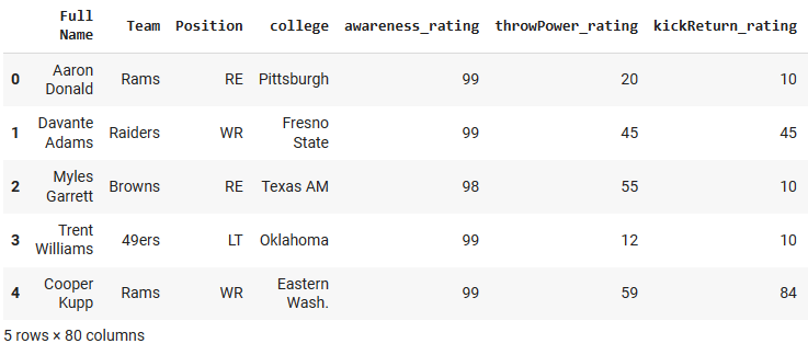
Fig 2: Our example dataset 

To keep things simple, we will only keep a few of the numerical features. The categorical features require encoding techniques and details that are not aligned with the scope of our discussion.

predictors = ["awareness_rating","throwPower_rating","kickReturn_rating",
              "leadBlock_rating","strength_rating","catchInTraffic_rating",
              "pursuit_rating", "catching_rating","acceleration_rating",
              "height","tackle_rating","yearsPro","throwUnderPressure_rating",
              "throwAccuracyDeep_rating","throwAccuracyShort_rating","speed_rating",
              "jumping_rating","toughness_rating","kickPower_rating",
              "kickAccuracy_rating","agility_rating","passBlock_rating","age"
             ]

csv[predictors].dtypes

awareness_rating            int64

throwPower_rating          int64

kickReturn_rating            int64

Now we will define our target.

target = "totalSalary"

Now we will setup the models we will use

from sklearn.linear_model import LinearRegression
from sklearn.neighbors import KNeighborsRegressor
from sklearn.ensemble import RandomForestRegressor
from tensorflow import keras
from tensorflow.keras import layers
from tensorflow.keras.callbacks import EarlyStopping

After importing the above dependencies and before we initialise our machine learning models, we applied preprocessing steps to scale and standardise the data and perform routine train/test splits, kindly note that these steps are omitted to keep the article easy to read from start to finish. The train/test split resulted in training data stored in variables "x_train" and "y_train", validation data "x_valid" and "y_valid" and lastly test data "x_test" and "y_test".

We move on to setting up each of the models we will be working with today.

lm = LinearRegression()
rf = RandomForestRegressor()
knn = KNeighborsRegressor(n_neighbors=10)
dnn = keras.Sequential([
    layers.Dense(units=30,activation="relu",input_shape=[scaled_data.shape[1]]),
    layers.Dense(units=20,activation="relu"),
    layers.Dropout(0.3),
    layers.Dense(units=10,activation="relu"),
    layers.Dense(units=1)
])

Then we will fit each model

#Fitting the linear regression
lm.fit(x_train,y_train)

#Fitting the k-nearest neighbor regressor
knn.fit(x_train,y_train)

#Fitting the random forest model
rf.fit(x_train,y_train)

#Fitting the deep neural network
early_stopping = EarlyStopping(
    min_delta=0.001,
    patience=20,
    restore_best_weights=True
)

dnn.compile(optimizer="adam",loss="mae")

dnn.fit(
    x_train,y_train,
    validation_data=(x_validation,y_validation),
    batch_size = 60,
    epochs=100,
    verbose=0,
    callbacks=[early_stopping]
)

Global Explanations

We will start with global explanations for our linear regression model. The technique we will use is permutation importance. It is a black-box global explanation technique.

import eli5
from sklearn.metrics import mean_squared_error
from eli5.sklearn import PermutationImportance
from eli5.permutation_importance import get_score_importances

Let's Get Global Explanations For Linear Regression Model

permutation = PermutationImportance(lm).fit(x_test,y_test)
eli5.show_weights(permutation,feature_names = predictors)

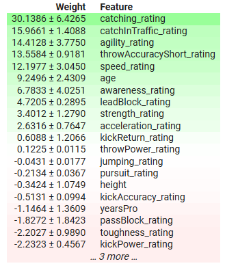
Fig 3: Global Explanations for Our Linear Regression Model

Let's interpret the results together. Permutation importance assumes that each of the columns in the dataset are independent. Therefore, it believes that it can alter one column at a time to observe the change in the model's error metrics and use that to decide which features are important. If the feature was important then shuffling its values will cause the model's error metrics to increase, and conversely if the feature wasn't important then the model's error metrics will actually decrease after shuffling the values in that column. In cases whereby the assumption of independence does not hold true then we must interpret these results with a grain of salt.

In the table above important features have positive coefficients and unimportant features have negative coefficients. "yearsPro", which is the years of experience the athlete possess, has a negative coefficient, but we know that in truth it matters, has our model discovered a phenomenon we are not aware of or is our explainer not giving us a faithful representation of the truth? 

Permutation importance may shuffle an athlete's experience unrealistically potentially making them too young for their level of expertise or having more experience than their total age. Additionally, this method ignores any interactions that may be present in the dataset, and credits all the changes in the model's error to that feature alone. Therefore, its results may be potentially unrealistic, emphasizing the need for caution and understanding the algorithm opposed to blindly applying it.
However, in the long run it can serve us valuable insight into the model's most important features, in this case the athlete's ability to catch and his agility are some of the most important features. And this makes sense because in football you are expected to be able to catch wide passes from your teammates, even if you are under a lot of pressure. Furthermore, after catching the ball, you have to avoid as many of your competitors as possible without dropping the ball, so therefore the importance placed on these features makes sense.

Local Explanations

As we stated earlier, local explanations help us understand how each feature affected each individual prediction our model is making,

We will get local explanations for our Deep Neural Network's expectations for Richard LeCounte's salary.

Fig 4: Richard LeCounte III

First, we import LIME.

LIME is an acronym for Locally Interpretable Model-Agnostic Explanations. It will explain which features contributed to the model’s output, and whether those contributions were pushing the output up or down. 

import lime
from lime import lime_tabular

explainer = lime_tabular.LimeTabularExplainer(training_data = np.array(x_train),mode='regression',feature_names=predictors)
exp = explainer.explain_instance(data_row=scaled_data.iloc[test],predict_fn=lm.predict)
exp.show_in_notebook(show_table=True)

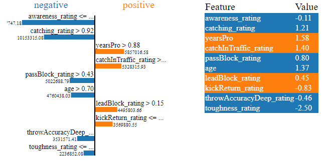
Fig 5: LIME Explanations For Our Deep Neural Network's Salary Expectations for Richard LeCounte's Salary

The plots above have a lot of information for us, first of all we can see which of LeCounte's physical abilities increased his expected salary and which decreased it. Our neural network expected LeCounte's toughness rating to lower his expected salary, this makes sense because LeCounte has an average toughness rating.  Furthermore, the deep neural network correctly identified LeCounte's strengths and expected his salary to increase on account of LeCounte's strengths. This is the how we would expect our model to function. Local explanations are powerful tools to validate our model instead of trusting it blindly.

Model Agnostic Explanations and Model Specific Explanations

In instances whereby we are aware of the underlying model’s structure, we can use explanation techniques designed specifically for that model architecture. These are commonly referred to as white-box explainers. In practice white-box explainers can be more computationally efficient than their black-box counterparts.

Black-box explainers are model-agnostic, meaning they can interpret and explain any model presented to them. The LIME algorithm we just covered is an example of a black-box explainer, it’s in the name (Locally Interpretable Model-Agnostic Explanations) 

Using white-box explainers when we are certain of the underlying model’s structure may help us render more faithful explanations of our model’s behaviour. Whereas black-box explainers are likely to introduce some levels of bias when explaining our models. Black-box explainers make some simplifying assumptions about the form of the model they are dealing with, if these assumptions are violated then the black-box explainer becomes unreliable.

As a rule of thumb, if you are certain of the model’s underlying properties you may be better off in the long run using white-box explainers. 

Let us take a look at a black-box explainer in action, the SHAP library has implementations of SHAP black-box explainers. We will demonstrate one below. 

Import SHAP

import shap

Calculate SHAP values

explainer = shap.Explainer(xgb.predict,scaled_data.loc[test:test_end,predictors])
shap_values = explainer(scaled_data.loc[test:test_end,predictors])

Plot our black-box explanations

shap.plots.beeswarm(shap_values)

Fig 6: SHAP black-box explanations for our XGB model

The width of each row is determined by outliers and doesn't convey any information about the feature's importance. We assess feature importance by considering the vertical placement of each feature along the plot. The higher up the feature is, the more important it was perceived by the SHAP algorithm.

Furthermore, notice that on some features blue and pink dots are well separated, whereas on other rows the blue and pink dots are jumbled together. When the dots are jumbled together this is usually a sign of an interaction effect between that feature and another feature or set of features. In brief, SHAP plots help us summarise a lot of information into just one plot. 

Each dot represents the Shapley value for each of our datapoints. This allows us to quickly understand how each individual datapoint affected the model's prediction on a granular level. The colour of each dot represents the direction and magnitude of influence that datapoint had on our model's prediction. Blue indicating a decrease in the model's output and pink indicates an increase. Keep in mind the SHAP algorithm assumes the features are independent, or in other words it ignores any interactions in the dataset. Violations of this assumption may make the algorithm unreliable. 

We will now consider a white-box explainer that is designed for tree-based models such as our XGB model. We use the special TreeExplainer() method designed to explain tree-based models.

tree_explainer = shap.TreeExplainer(xgb)
tree_shap_values = explainer(x_test)

Then we can plot the white-box explanations

shap.plots.beeswarm(tree_shap_values)

Fig 7: SHAP white-box explanations for our XGB model

Compare the top 4 most important features from the black-box SHAP explanation and the white-box SHAP explanation, can you see the disagreement problem in action? 

Defining The Disagreement Problem and Factors Contributing to The Problem

So now that we understand what model explanations are, we can now begin focusing more on the disagreement problem directly. Let’s start by reviewing what is a disagreement.
Let's dissect what constitutes a disagreement in the realm of feature importance explanations:

• Feature Permutations: The first form of disagreement is when feature permutations differ. If the specific order of feature importance holds weight in your workflow, the emergence of different permutations across explanations becomes a pivotal point of contention. This aspect becomes particularly crucial when the nuanced sequencing of features carries significance for your analysis.
• Best Ranked Feature Sets: Diving deeper, the disagreement extends to the best-ranked feature sets. When the strict adherence to the exact permutation of feature importance is relaxed, attention shifts to the set of top features. A disparity in the top 3, 5, or any 'n' features identified by different explainers for the same model becomes a noteworthy point of divergence in your analytical journey.
• Coefficient Sign Fluctuation: The heartbeat of many explainers lies in the coefficients assigned to features, indicating their positive or negative contribution toward the desired outcome. A change in the sign of this coefficient between two explanations for the same model stands as a flag in your workflow. Such fluctuations serve as indicators of disagreement, urging a closer inspection of the model's inner workings.
• Relative Ordering Amongst Features of Interest: Zooming in on specific features of interest, the disagreement takes on yet another dimension. If your focus is on benchmarking the importance of a particular feature relative to another, shifts in the order of these two features across different explanations become the battleground of disagreement in your workflow.

What Isn't a Disagreement?

It's just as crucial to recognize that not all disparities signify disagreement. Let's explore instances where explanations maintain a harmonious coexistence:

• Divergent Importance Values: Explanations refrain from true disagreement when the feature importance values, as calculated by different explainers, don't align precisely. The crux lies in the acknowledgment that diverse algorithms yield distinct calculations, making direct comparisons challenging. The emphasis here is not on the numerical equality of importance values but on the consistent insights derived from disparate explanations.
• Consistent Insights Over Exact Values: The essence of non-disagreement is rooted in the pursuit of consistent insights rather than an obsessive quest for exact numerical parity. The goal is not to demand that every explainer precisely mirrors the importance values of its counterparts. Instead, the focus shifts to the broader narrative — ensuring that the explanations, though numerically distinct, converge in guiding us towards consistent and reliable model insights.
• Model Complexity and Estimation Challenges: As the tapestry of model complexity unfolds, a fundamental truth emerges: the difficulty of accurately estimating the inner workings of the model grows in direct proportion. Non-disagreement is a recognition of this inherent complexity. In the face of intricate models, the divergence in explanation values becomes an expected challenge rather than a cause for alarm. This perspective aligns with the evolving nature of AI, where the pursuit of transparency encounters growing intricacies.

Why Do Explainers Disagree With Each Other?
There are many reasons why explainers may disagree with each other, let’s try to make sense of a few cases together.

Comparing Global And Local Explainers

One reason why we may observe disagreements is because we may be comparing global and local explanations. Whilst this is a very simple mistake to make, I would like to believe that none of the readers of this article should go on to make that mistake. Global and local explanations cannot be easily compared directly to each other. Unless you have a detailed understanding of how the algorithms are implemented under the hood, comparing global and local explanations is not advisable and doing so will probably yield divergent explanations.

Comparing Black-Box And White-Box Explainers

Furthermore, another deceivingly benign source of disagreements could be comparing black-box and white-box explainers. Remember black-box explainers are trying to render the utility of being able to explain any algorithm, therefore they make certain simplifying assumptions about the model or the model’s behaviour. These assumptions that the black-box explainer makes allow it to be robust and work well under a wide range of circumstances, however when the assumptions aren’t true then the explainer introduces bias. This bias may cause the black-box and white-box explanations to differ. 

Changing The Order of Features

Our troubles do not end here, a cunning cause for disagreements may be any changes to the order in which the features are presented. Some explanation techniques are sensitive to the order of the model inputs while some aren’t. For example, Mutual Information is not sensitive to the order of inputs, but SHAP is! Therefore, it may be possible that a SHAP explainer may fail to agree with itself after observing identical models.  

For example below we output two SHAP explanations we got from two identical XGBRegressors. The only difference between the two models is the order of the features they take as inputs, beyond that they are learning from the same dataset, and have the same target. 

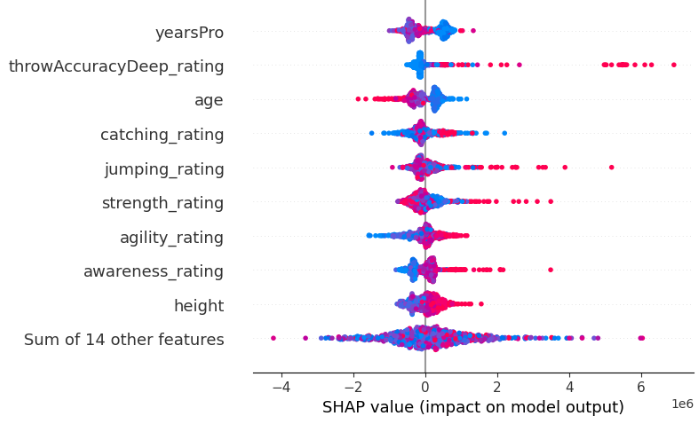
Fig 8 : Our Initial SHAP Values

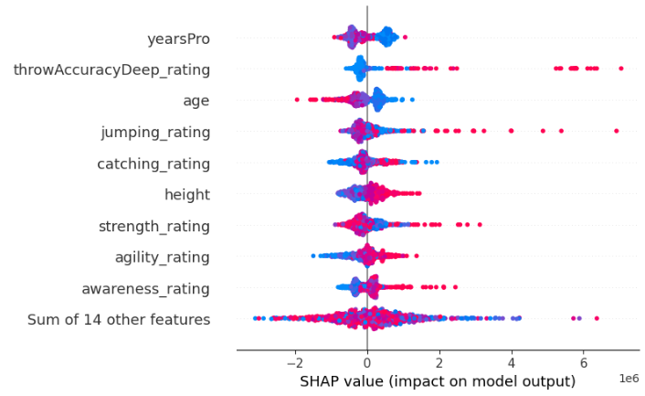
Fig 9: SHAP Values After Changing Feature Order

After shuffling the order that the features are shown to the model, we can see that our explanations now disagree with each other. The height feature has suddenly risen in importance even though there was no new information presented. The top 3 remained unchanged, but most features jumped up and down and changed positions. If you plan on using bootstrapping techniques or other forms of resampling or subset-selection, then you should at least be aware that this phenomenon is normal and expected. 

Moreover, different implementations of the same explanation technique may fail to agree with each other because of the slight differences in their calculations. For example, eli5’s implementation of Permutation Importance is sensitive to the order of inputs but sklearn’s implementation of the same explanation technique is not. This is possible because the same explanation technique can be implemented in a variety of ways. 

To demonstrate that eli5's implementation of Permutation Importance is sensitive to the order of inputs, below we output two explanations obtained using eli5's implementation of Permutation Importance. We obtained the results from two identical XGBRegressors. The only difference between the two models is the order of the features they take as inputs, beyond that they are learning from the same dataset, and have the same target. 

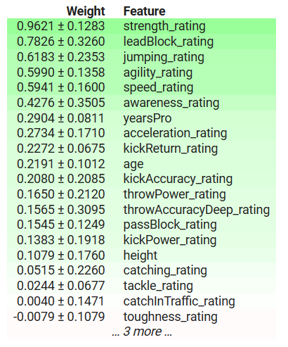
Fig 10: Initial Permutation Importance

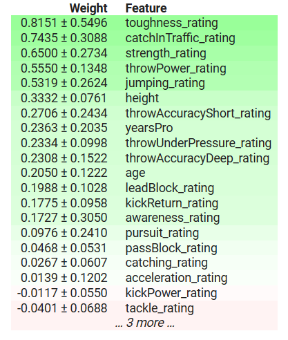
Fig 11: Shuffled Permutation Importance

Observe that "kickPower_rating" initially had a positive coefficient but after changing the order of the features it now has a negative coefficient! Such volatile fluctuations are considered strong disagreements. The most important features changed, the relative order between the features has also changed.

Lastly, one of the elephants in the room is likely to be methodological divergence—a pivotal factor giving rise to the intriguing phenomenon of explainers disagreeing with each other though they are both explaining the same model. Because each explainer calculates different metrics about the model, they may each interpret the model in different light.

Fortunately for us, XGB has an implemented function that allows us to assess feature importance. Let's take advantage of that function to observe which explanation technique gives us a faithful representation of the truth. In order to help the reader, we have included the results of the previous explanations here so that you don’t have to keep scrolling up and down.

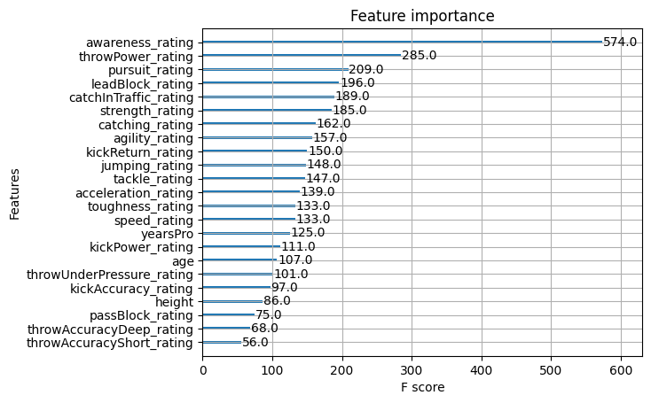
Fig 12: XGB Feature Importance

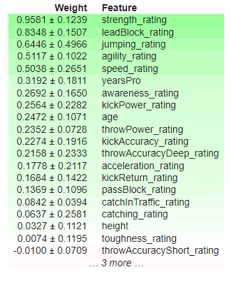
Fig 13: XGB Permutation Importance

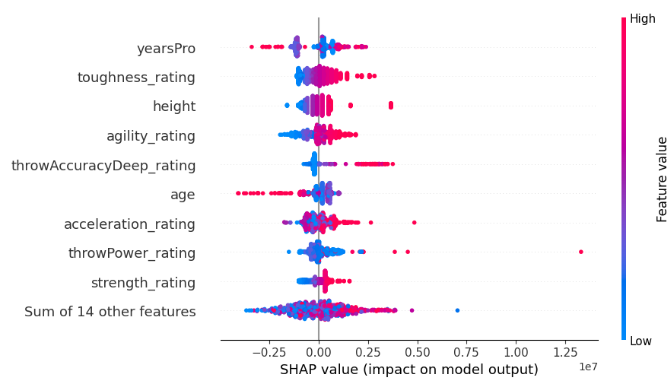
Fig 14: SHAP White-Box Explanations

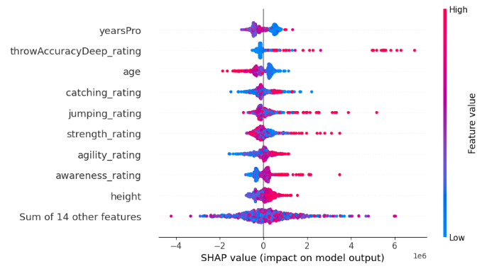
Fig 15: SHAP Black-Box Explanations

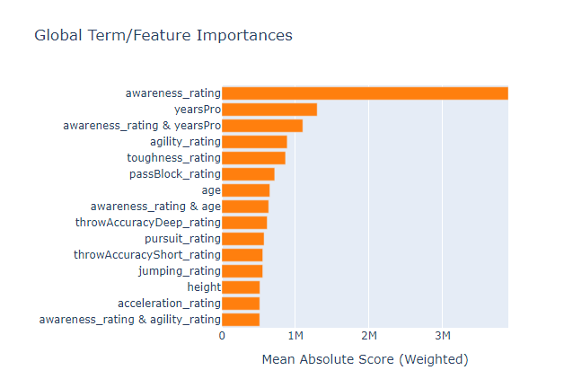
Fig 16: A Glass-Box Tree Based Model Feature Importance

Awareness rating was the most important feature to our model, however our small set of black-box explanation techniques failed to explain that to us, missing the top 3 features entirely. This is a sobering reminder that explanations are only estimates of feature importance, and not absolute truth. Furthermore, notice that "yearsPro" repeatedly ranked towards the top, but in truth it wasn't that important, this cautions us against a simplistic assumption that features that repeatedly rank high across different tests are inherently important. 

The black-box explainer we applied to our XGB model contradicts the white-box explainer we applied, but in the end both explainers were wrong. So, in a situation like this figuring out which explainer is more faithful would have been a complete waste of your time, because neither of them takes the reader any closer to the truth.

I also fit an explainable boosting machine on the data to see if the glass-box model could be used as a proxy for assessing feature importance, and whilst it managed to correctly identify the most important feature from the dataset, it may not always be a viable option especially if the model you're trying to explain isn't a tree-based model. Unfortunately, however, the glass-box model also found the "yearsPro" feature to be informative even though it wasn't, this means that we should also be aware that our explainers may agree on false information!

Case Study

We are now ready to begin working with real market data, we begin by extracting data from the MetaTrader 5 Terminal. Our strategy involves developing a MetaQuotes Language 5 (MQL5) script tailored for efficient data extraction and transformation. We begin by declaring global variables.

//---Our handlers for our indicators
int ma_handle;
int rsi_handle;
int cci_handle;
int ao_handle;
int bbands_handle;
int atr_handle;

Following this, we will create arrays to store the values of our technical indicators. These data structures assume a pivotal role in methodically capturing, managing, and leveraging the outputs of the indicators throughout the entirety of the script execution. 

//---Data structures to store the readings from our indicators
double ma_reading[];
double rsi_reading[];
double cci_reading[];
double ao_reading[];
double bb_high_reading[];
double bb_low_reading[];
double bb_mid_reading[];
double atr_reading[];

Subsequently, we need to create a name for our CSV file. 

//---File name
string file_name = "The Dissagrement Problem Data.csv";

From there, we need to create a variable to store how many bars we would like to request.

//---Amount of data requested
int size = 10000;
int size_fetch = size + 50;

Moving on to setting up our technical indicator handlers. Each time we setup a technical indicator we need to specify the Symbol we are going to be using it on and the timeframe we intend to use. From there depending on the indicator, you may need to specify the period of the indicator, the shift parameter, the smoothing method and which price should the indicator be applied to 

void OnStart()
  {
      //---Setup our technical indicators
      ma_handle = iMA(_Symbol,PERIOD_CURRENT,20,0,MODE_EMA,PRICE_CLOSE);
      rsi_handle = iRSI(_Symbol,PERIOD_CURRENT,60,PRICE_CLOSE);
      cci_handle = iCCI(_Symbol,PERIOD_CURRENT,10,PRICE_CLOSE);
      ao_handle = iAO(_Symbol,PERIOD_CURRENT);
      bbands_handle = iBands(_Symbol,PERIOD_CURRENT,120,0,0.2,PRICE_CLOSE);
      atr_handle = iATR(_Symbol,PERIOD_CURRENT,14);

Continuing the script execution, the subsequent responsibility involves the transference of values from our indicator handles to the designated data structures.

 //---Set the values as series
      CopyBuffer(ma_handle,0,0,size_fetch,ma_reading);
      ArraySetAsSeries(ma_reading,true);
      CopyBuffer(rsi_handle,0,0,size_fetch,rsi_reading);
      ArraySetAsSeries(rsi_reading,true);
      CopyBuffer(cci_handle,0,0,size_fetch,cci_reading);
      ArraySetAsSeries(cci_reading,true);
      CopyBuffer(ao_handle,0,0,size_fetch,ao_reading);
      ArraySetAsSeries(ao_reading,true);
      CopyBuffer(bbands_handle,0,0,size_fetch,bb_mid_reading);
      ArraySetAsSeries(bb_mid_reading,true);
      CopyBuffer(bbands_handle,1,0,size_fetch,bb_high_reading);
      ArraySetAsSeries(bb_high_reading,true);
      CopyBuffer(bbands_handle,2,0,size_fetch,bb_low_reading);
      ArraySetAsSeries(bb_low_reading,true);
      CopyBuffer(atr_handle,0,0,size_fetch,atr_reading);
      ArraySetAsSeries(atr_reading,true);

Before we begin the file-writing process, a crucial preliminary task involves the incorporation of a file handler within our script. This foundational step encompasses the configuration of requisite parameters and mechanisms to enable the smooth creation and manipulation of the output file.

      //---Write to file
       int file_handle=FileOpen(file_name,FILE_WRITE|FILE_ANSI|FILE_CSV,",");

Following this, a critical phase in our script unfolds as we systematically navigate through the arrays of historical prices and indicator values so we can encode the data to our designated CSV file.

for(int i=-1;i<=size;i++){
      if(i == -1){
            FileWrite(file_handle,"Time","Open","High","Low","Close","MA 20","RSI 60","CCI 10","AO","BBANDS 120 MID","BBANDS 120 HIGH","BBANDS 120 LOW","ATR 14");
      }
      
      else{
            FileWrite(file_handle,iTime(_Symbol,PERIOD_CURRENT,i),
                                 iOpen(_Symbol,PERIOD_CURRENT,i),
                                 iHigh(_Symbol,PERIOD_CURRENT,i),
                                 iLow(_Symbol,PERIOD_CURRENT,i),
                                 iClose(_Symbol,PERIOD_CURRENT,i),
                                 ma_reading[i],
                                 rsi_reading[i],
                                 cci_reading[i],
                                 ao_reading[i],
                                 bb_mid_reading[i],
                                 bb_high_reading[i],
                                 bb_low_reading[i],
                                 atr_reading[i]);
      }
    }
    FileClose(file_handle);
  }

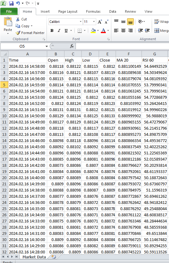
Fig 17: Market Data from the MetaTrader 5 Terminal

We’re now ready to handle the data and apply our new skills that we learned from the example dataset. 

We now import our dependencies.

#Import Dependencies
import pandas as pd
import numpy as np
import matplotlib.pyplot as plt
import shap
import lime
from lime import lime_tabular
import eli5
from eli5.sklearn import PermutationImportance
from sklearn.feature_selection import mutual_info_regression

Loading dependencies for IntepretML.

from interpret import set_visualize_provider
from interpret.provider import InlineProvider
set_visualize_provider(InlineProvider())
from interpret import show
from interpret.blackbox import MorrisSensitivity

Read in the csv.

csv = pd.read_csv("/enter/your/path/here")

Let's setup the target.

csv["Target"] = csv["Close"].shift(-30)

Drop any rows with missing values.

csv.dropna(axis=0,inplace=True)

Let's create a list of predictors.

drop = ["Time","Target"]
predictors = csv.columns.tolist()
predictors = [col for col in predictors if col not in drop]
predictors

Let's scale the data.

from sklearn.preprocessing import StandardScaler
scaler = StandardScaler()
print(scaler.fit(csv.loc[:,predictors]))
scaled_data =  pd.DataFrame(scaler.transform(csv.loc[:,predictors]), index = csv.index, columns = predictors)
scaled_data

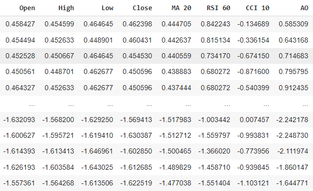
Fig 18:  Scaled Market Data

Setting up our black box algorithms

#Black box models
from xgboost import XGBRegressor
from sklearn.linear_model import LinearRegression
from xgboost import plot_importance
from tensorflow import keras
from tensorflow.keras import layers
from tensorflow.keras.callbacks import EarlyStopping

Train/Test Split

train = 0
train_end = 5000
test = train_end + 40

Setting Up Our Linear Model

lm = LinearRegression()
lm.fit(scaled_data.loc[train:train_end,predictors],csv.loc[train:train_end,"Target"])

Setting up our XGB Model

#XGBModel
xgb = XGBRegressor()
xgb.fit(scaled_data.loc[train:train_end,predictors],csv.loc[train:train_end,"Target"])

Setting Up Our Deep Neural Network Model

dnn = keras.Sequential([
    layers.Dense(units=30,activation="relu",input_shape=[scaled_data.shape[1]]),
    layers.Dense(units=20,activation="relu"),
    layers.Dropout(0.3),
    layers.Dense(units=10,activation="relu"),
    layers.Dense(units=1)
])

early_stopping = EarlyStopping(
    min_delta=0.001,
    patience=20,
    restore_best_weights=True
)

dnn.compile(optimizer="adam",loss="mae")

dnn.fit(
    scaled_data.loc[train:train_end,predictors],csv.loc[train:train_end,"Target"],
    validation_data=(csv.loc[validation:validation_end,predictors],csv.loc[validation:validation_end,"Target"]),
    batch_size = 60,
    epochs=100,
    verbose=0,
    callbacks=[early_stopping]
)

Getting Global Explanations For Our Deep Neural Network

We will use the alibi package to get explanations for our deep neural network. The alibi package has a useful implementation of an explanative technique known as Accumulated Local Effects (ALE). ALE extends on all the explanative techniques we have considered so far because it is robust and can handle strongly correlated features, it relaxes assumptions of feature independence, it can be visually interpreted, it is computationally efficient and unlike some other explanation techniques, ALE does not rely on linearity assumptions, making it well-suited for capturing complex relationships in the data.   

First we calculate our ALE values.

dnn_ale = ALE(dnn.predict, feature_names  = predictors,target_names=["Close 30 Steps"])

Then we convert our input data into NumPy format before we can obtain our ALE plots.

X = scaled_data.loc[train:train_end,predictors].to_numpy()
dnn_alibi =dnn_ale.explain(X)
plot_ale(dnn_alibi,n_cols=4, fig_kw={'figwidth': 20, 'figheight': 10}, sharey=None)

ALE plots help us interpret how changes in each feature affect the model's output, for example below we have the ALE plot for our Awesome Oscillator. As we can observe, the Awesome Oscilator can help our deep neural network anticipate when price will fall, we observe the downward slope in the ALE plot as the Awesome Oscillator value increases.

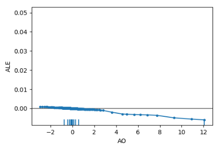
Fig 19: ALE Plot For Our Awesome Oscillator

Furthermore, features that aren't informative will have an ALE plot that resembles a horizontal line, meaning that changes in that feature have little impact on the target. In our case study the Relative Strength Index wasn't informative. 

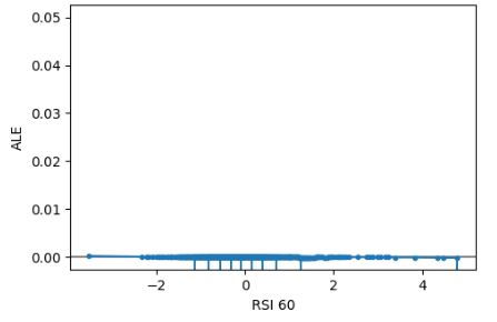
Fig 20 : ALE RSI

Getting Global Explanations From Model Agnostic SHAP Explainer

explainer = shap.Explainer(xgb.predict,scaled_data.loc[test:,predictors])
shap_values = explainer(scaled_data.loc[test:,predictors])
shap.plots.beeswarm(shap_values)

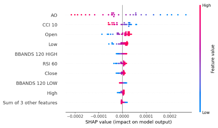
Fig 21:  SHAP Black-box Beeswarm plot of our XGB model

Our beeswarm plot informs us the Awesome Oscillator is the most important feature in this dataset, remember that the width of each row in the plot does not convey any information because it can be determined simply by outliers. Furthermore, we notice that the blue and pink dots don't appear to be jumbled up, meaning that the dataset may not have strong interaction terms in it.

Feature Importance According to Mutual Information

mi_scores = mutual_info_regression(scaled_data.loc[test:,predictors], csv.loc[test:,"Target"])
mi_scores = pd.Series(mi_scores, name="MI Scores", index=scaled_data.columns)
mi_scores = mi_scores.sort_values(ascending=False)
mi_scores

BBANDS 120 MID     1.739039

BBANDS 120 HIGH    1.731220

BBANDS 120 LOW     1.716019

MA 20                      1.525800

High                        1.172096

Open                       1.155583

Close                       1.143642

Low                         1.140613

ATR 14                     0.421772

AO                           0.232608

RSI 60                      0.181932

CCI 10                     0.016491

Mutual information completely disagrees with our SHAP explainer as far as the top 4 features are concerned. This only casts more doubts on our already confusing journey, to make matters worse our SHAP was explainer was actually correct about the Awesome Oscillator being the most important feature in this case. Therefore, relying on multiple explainers is actually a double-edged sword, on one side it protects you against the bias inherited from any explanation used but on the other hand it creates a larger probability space for disagreements to crop up.  It is difficult to say which case is empirically better, because it all depends on the particular dataset, the particular model and so many other variables.

Lastly, we will consider Morris Sensitivity Analysis as our final Global Black-Box Explainer

msa = MorrisSensitivity(xgb, scaled_data.loc[train:train_end,predictors])
show(msa.explain_global())

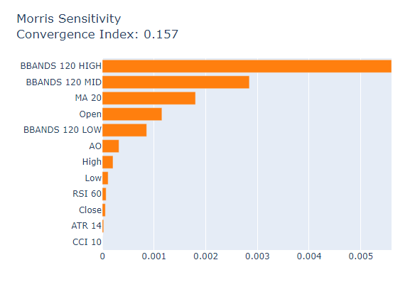
Fig 22: Morris Sensitivity Analysis

Here's the actual importance metrics from our XGB model.

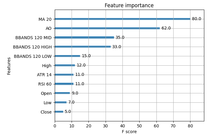
Fig 23: XGB Market Data Importance

The moving average was the most important feature in our dataset, followed by the Awesome Oscillator. So, in this particular case, Morris Sensitivity Analysis gave us the best explanations relatively speaking, however in most cases you may not have access to the ground truth, therefore how would you have selected which explanation to give more weight? How confident would you have been in your decision? How could you validate any of your decisions regarding feature importance if you didn't have access to the true feature importance tables? 

Conclusion

As we can see there are no simple answers here, there are just too many moving parts. The form and structure of your datasets has to be taken into consideration, the underlying model also has to be taken into consideration, the presence of interactions terms in your data has to be accounted for and above all the innerworkings of each explanation has to be at the fingertips of the machine learning practitioner. Furthermore, in our controlled exampled we observed that it is possible for all of your explainers to be wrong, therefore in such a situation trying to resolve any disagreements would have been a futile waste of time. Therefore, the payoff we get from explanative techniques does not always justify the complexity they may introduce. However, as time progresses, we may realise better explanative techniques and observe better algorithms.

Recommendation

Therefore, after taking all this into consideration I am convinced that possibly the best solution to the disagreement problem may be to rely more on machine learning models that are interpretable like Generalised Additive Models (GAM) or Explainable Boosting Machines (EBM), such models perfectly substitute the need for explanations. As of today, there aren't any globally recognised solutions to every possible case of the disagreement problem, but as awareness on the issue continues to grow maybe one day we will be able to confidently explain any machine learning model we build.