Reimagining Classic Strategies (Part XI): Moving Average Cross Over (II)

We have previously covered the idea of forecasting moving average cross-overs, the article is linked here. We observed that moving average cross-overs are easier to forecast than price changes directly. Today we will revisit this familiar problem but with an entirely different approach.
 
We now want to thoroughly investigate how big of a difference this makes for our trading applications and how this fact can improve your trading strategies. Moving averages cross-overs are one of the oldest existing trading strategies. It is challenging to build a profitable strategy using such a widely known technique. Nevertheless, I hope to show you in this article that old dogs can indeed learn new tricks.

To be empirical in our comparisons, we will first build a trading strategy in MQL5 for the EURGBP pair using just the following indicators:

1. 2 Exponential Moving Averages applied to the Close Price. One with a period of 20, and the other set to 60.
2. The Stochastic oscillator with the default settings of 5,3,3 applied set to Exponential Moving Average Mode and set to make its calculations in the CLOSE_CLOSE mode
3. The Average True Range indicator with a period of 14 to set our take-profit and stop-loss levels.
   

Our strategy will be intended to trade the Daily Time Frame. We will back test this strategy from the first of January 2022 until the beginning of June 2024. Our strategy will initially use classical trading rules. So, buy signals will be generated whenever the fast-moving average crosses above the slow-moving average and the stochastic reading is above 80. And the converse is true for our sell signals. We will register a sell signal when the fast-moving average is beneath the slow, and the stochastic oscillator is beneath 20.

We will extensively explore the parameters under which the back test was performed later in the article. However, we will take note of key performance metrics over the back test, such as the Sharpe ratio, proportion of profitable trades, max profit and other important performance metrics.

Once complete, we will then carefully replace all the legacy trading rules with algorithmic trading rules learned from our market data. We will train 3 AI models to learn to forecast:

1. Future Volatility: This will be done by training an AI model to forecast the ATR reading.
2. Relationship between change in price and the moving average cross-overs : We will create 2 discrete states that the moving averages can be in. The moving averages can only be in 1 state at a time. This will help our AI model focus on the critical changes in the indicator and the average effect of these changes on future price levels.
   
3. Relationship between the change in price and the stochastic oscillator: This time we will create 3 discrete states, that the stochastic oscillator can only occupy 1 at a time. Our model will then learn the average effect of the critical changes in the stochastic oscillator.

These 3 AI models will not be trained on any of the time periods we will use for our back test. Our back test will run from 2022 until June 2024, and our AI models will be trained from 2011 until 2021. We made sure not to overlap the training and back testing, so we can try our best to remain close to the model’s true performance on data it has not seen.

Believe it or not, we successfully improved all performance metrics across the board. Our new trading strategy was more profitable, had an increased Sharpe ratio and won more than half, 55%, of all the trades it placed during the back test period.

If such an old and widely exploited strategy can be made more profitable, I believe this should encourage any reader that their strategies can also be made more profitable, if you can only frame your strategy the right way.

Most traders work hard over long periods of time to create their trading strategies and will hardly ever discuss their prized personal strategies at length. Therefore, the moving average cross-over serves a neutral point of discussion that all members of our community can use as a benchmark. I hope to provide you a generalized framework which you can supplement with your own trading strategies and by following this framework accordingly, you should see some improvements to your own strategies.

Getting Started

To get started, we will launch our MetaEditor IDE and get started by building a trading application that will serve as our baseline.

We want to implement a simple moving average cross over strategy, so let's get started. We will import the trade library first.

//+------------------------------------------------------------------+
//|                                         EURGBP Stochastic AI.mq5 |
//|                                        Gamuchirai Zororo Ndawana |
//|                          https://www.mql5.com/en/gamuchiraindawa |
//+------------------------------------------------------------------+
#property copyright "Gamuchirai Zororo Ndawana"
#property link      "https://www.mql5.com/en/gamuchiraindawa"
#property version   "1.00"

//+------------------------------------------------------------------+
//| Libraries                                                        |
//+------------------------------------------------------------------+
#include <Trade\Trade.mqh>
CTrade Trade;

Define global variables.

//+------------------------------------------------------------------+
//| Global variables                                                 |
//+------------------------------------------------------------------+
double vol,bid,ask;

Creating handlers for our technical indicators.

//+------------------------------------------------------------------+
//| Technical indicator handlers                                     |
//+------------------------------------------------------------------+
int slow_ma_handler,fast_ma_handler,stochastic_handler,atr_handler;
double slow_ma[],fast_ma[],stochastic[],atr[];

We will also fix some of our variables as constants.

//+------------------------------------------------------------------+
//| Constants                                                        |
//+------------------------------------------------------------------+
const int slow_period = 60;
const int fast_period = 20;
const int atr_period = 14;

Some of our inputs should be controlled manually. Such as the lot size and the width of the stop loss.

//+------------------------------------------------------------------+
//| User inputs                                                      |
//+------------------------------------------------------------------+
input group "Money Management"
input int lot_multiple = 5; //Lot size

input group "Risk Management"
input int atr_multiple = 5; //Stop Loss Width

When our system is loading, we will call a special function to set up our technical indicators and save market data.

//+------------------------------------------------------------------+
//| Expert initialization function                                   |
//+------------------------------------------------------------------+
int OnInit()
  {
//--- Setup our technical indicators and fetch market data
   setup();

//---
   return(INIT_SUCCEEDED);
  }

Otherwise, if we are no longer using the trading application, let us free up the resources we do not need anymore.

//+------------------------------------------------------------------+
//| Expert deinitialization function                                 |
//+------------------------------------------------------------------+
void OnDeinit(const int reason)
  {
//---
   IndicatorRelease(fast_ma_handler);
   IndicatorRelease(slow_ma_handler);
   IndicatorRelease(atr_handler);
   IndicatorRelease(stochastic_handler);
  }

If we have no open positions in the market, we will look for a trading opportunity.

//+------------------------------------------------------------------+
//| Expert tick function                                             |
//+------------------------------------------------------------------+
void OnTick()
  {
//--- Fetch updated quotes
   update();

//--- If we have no open positions, check for a setup
   if(PositionsTotal() == 0)
     {
      find_setup();
     }
  }

This function will initialize our technical indicators and save the lot size the end user specified.

//+------------------------------------------------------------------+
//| Setup technical market data                                      |
//+------------------------------------------------------------------+
void setup(void)
  {
//--- Setup our indicators
   slow_ma_handler    = iMA("EURGBP",PERIOD_D1,slow_period,0,MODE_EMA,PRICE_CLOSE);
   fast_ma_handler    = iMA("EURGBP",PERIOD_D1,fast_period,0,MODE_EMA,PRICE_CLOSE);
   stochastic_handler = iStochastic("EURGBP",PERIOD_D1,5,3,3,MODE_EMA,STO_CLOSECLOSE);
   atr_handler        = iATR("EURGBP",PERIOD_D1,atr_period);
//--- Fetch market data
   vol = lot_multiple * SymbolInfoDouble("EURGBP",SYMBOL_VOLUME_MIN);
  }

We will now build a function to save updated price offers when we receive them.

//+------------------------------------------------------------------+
//| Fetch updated market data                                        |
//+------------------------------------------------------------------+
void update(void)
  {
//--- Update our market prices
   bid = SymbolInfoDouble("EURGBP",SYMBOL_BID);
   ask = SymbolInfoDouble("EURGBP",SYMBOL_ASK);
//--- Copy indicator buffers
   CopyBuffer(atr_handler,0,0,1,atr);
   CopyBuffer(slow_ma_handler,0,0,1,slow_ma);
   CopyBuffer(fast_ma_handler,0,0,1,fast_ma);
   CopyBuffer(stochastic_handler,0,0,1,stochastic);
  }

This function will finally check for our trading signal. If the signal is found, we will enter our positions with stop losses and take profits set up by the ATR.

//+------------------------------------------------------------------+
//| Check if we have an oppurtunity to trade                         |
//+------------------------------------------------------------------+
void find_setup(void)
  {
//--- Can we buy?
   if((fast_ma[0] > slow_ma[0]) && (stochastic[0] > 80))
     {
      Trade.Buy(vol,"EURGBP",ask,(ask - (atr[0] * atr_multiple)),(ask + (atr[0] * atr_multiple)),"EURGBP");
     }

//--- Can we sell?
   if((fast_ma[0] < slow_ma[0]) && (stochastic[0] < 20))
     {
      Trade.Sell(vol,"EURGBP",bid,(bid + (atr[0] * atr_multiple)),(bid - (atr[0] * atr_multiple)),"EURGBP");
     }
  }
//+------------------------------------------------------------------+

We are now ready to back-test our trading system. We will train the simple moving average cross over trading algorithm we have just defined above on the EURGBP Daily market data. Our back test period will be from the beginning of January 2022 until the end of June 2024. We will set the "Forward" parameter to false. The market data will be modeled using real ticks our Terminal will have to request from our broker. This will ensure our test results are closely emulating the market conditions that transpired on that day.

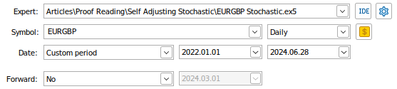
Fig1: Some of the settings for our back-test

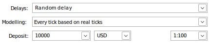
Fig 2: The remaining parameters of our back test

The results from our initial back-test are not encouraging. Our trading strategy was losing money over the entire test. However, this is not surprising either because we already know that the moving average cross-overs are delayed trading signals. Fig 3 below summarizes the balance of our trading account during the test.

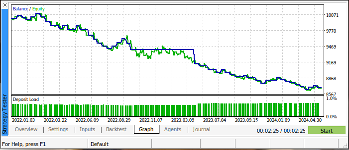
Fig 3: The balance of our trading account as we performed the back test

Our Sharpe ratio was -5.0, and we lost 69.57% of all the trades we placed. Our average loss was larger than our average profit. These are bad performance indicators. If we were to use this trading system in its current state, we would most certainly lose our money rapidly.

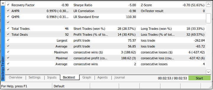
Fig 4: The details of our back-test using a legacy approach to trading the markets

Strategies relying on moving average cross-overs and the stochastic oscillator have been extensively exploited and are unlikely to have any material edge we can use as human traders. But, this does not imply there is no material edge our AI models can learn. We are going to employ a special transformation known as "dummy encoding" to represent the current state of the markets to our AI model.

Dummy encoding is used when you have an unordered categorical variable, and we assign one column for each value it can take. For example, image if the MQL5 team allowed you to decide which color theme you want your installation of MetaTrader 5 to be. Your options are Red, Pink or Blue. We can capture this information by having a database with 3 columns titled "Red","Pink" and "Blue" respectively. The column you selected during installation will be set to one, the other columns will remain 0. This is the idea behind dummy encoding.

Dummy encoding is powerful because if we had selected a different representation of the information, such as 1-Red, 2-Pink and 3-Blue, our AI Models may learn false interactions in the data that do not exist in real life. For example, the model may learn that 2 and a half may is the optimal color. Therefore, dummy encoding helps us present our models with categorical information in a manner that ensures the model does not implicitly assume there is a scale to the data it is being given.

Our moving averages will have two states, the first state will be activated when the fast-moving average is above the slow. Otherwise, the second state will be activated. Only one state can be active at any moment. It is impossible for price to be in both states at the same time. Likewise, our stochastic oscillator will have 3 states. One will be active if price is above the 80 reading on the indicator, the second will be activated when price is beneath the 20 region. Otherwise, the third state will be activated.

The active state will be set to 1 and all other states will be set to 0. This transformation will force our model to learn the average change in the target as price moves through the different states of our indicator. This is close to what professional human traders do. Trading is not like engineering, we cannot expect millimeter precision. Rather, the best human traders, overtime, learn what is most likely to happen next. Training our model using dummy encoding will drive us towards the same end. Our model will optimize its parameters to learn the average change in price, given the current state of the technical indicators.

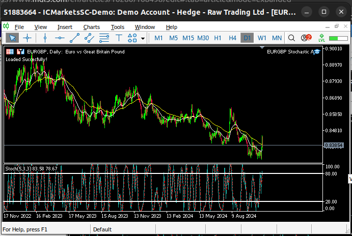
Fig 5: Visualizing the EURGBP Daily market

The first step we will take to build our AI models, is to fetch the data we need. It is always best practice to fetch the same data you will use in production. That is the reason we will use this MQL5 script to fetch all our market data from the MetaTrader 5 terminal. Unexpected differences between how the indicator values are being calculated in different libraries may leave us with unsatisfactory results at the end of the day.

//+------------------------------------------------------------------+
//|                                                      ProjectName |
//|                                      Copyright 2020, CompanyName |
//|                                       http://www.companyname.net |
//+------------------------------------------------------------------+
#property copyright "Gamuchirai Zororo Ndawana"
#property link      "https://www.mql5.com/en/users/gamuchiraindawa"
#property version   "1.00"
#property script_show_inputs

//+------------------------------------------------------------------+
//| Script Inputs                                                    |
//+------------------------------------------------------------------+
input int size = 100000; //How much data should we fetch?

//+------------------------------------------------------------------+
//| Global variables                                                 |
//+------------------------------------------------------------------+
int    ma_fast_handler,ma_slow_handler,stoch_handler,atr_handler;
double ma_fast[],ma_slow[],stoch[],atr[];

//+------------------------------------------------------------------+
//| On start function                                                |
//+------------------------------------------------------------------+
void OnStart()
  {
//--- Load indicator
   ma_fast_handler    = iMA(Symbol(),PERIOD_CURRENT,20,0,MODE_EMA,PRICE_CLOSE);
   ma_slow_handler    = iMA(Symbol(),PERIOD_CURRENT,60,0,MODE_EMA,PRICE_CLOSE);
   stoch_handler      = iStochastic(Symbol(),PERIOD_CURRENT,5,3,3,MODE_EMA,STO_CLOSECLOSE);
   atr_handler        = iATR(Symbol(),PERIOD_D1,14);

//--- Load the indicator values
   CopyBuffer(ma_fast_handler,0,0,size,ma_fast);
   CopyBuffer(ma_slow_handler,0,0,size,ma_slow);
   CopyBuffer(stoch_handler,0,0,size,stoch);
   CopyBuffer(atr_handler,0,0,size,atr);

   ArraySetAsSeries(ma_fast,true);
   ArraySetAsSeries(ma_slow,true);
   ArraySetAsSeries(stoch,true);
   ArraySetAsSeries(atr,true);

//--- File name
   string file_name = "Market Data " + Symbol() +" MA Stoch ATR " +  " As Series.csv";

//--- Write to file
   int file_handle=FileOpen(file_name,FILE_WRITE|FILE_ANSI|FILE_CSV,",");

   for(int i= size;i>=0;i--)
     {
      if(i == size)
        {
         FileWrite(file_handle,"Time","Open","High","Low","Close","MA Fast","MA Slow","Stoch Main","ATR");
        }

      else
        {
         FileWrite(file_handle,iTime(Symbol(),PERIOD_CURRENT,i),
                   iOpen(Symbol(),PERIOD_CURRENT,i),
                   iHigh(Symbol(),PERIOD_CURRENT,i),
                   iLow(Symbol(),PERIOD_CURRENT,i),
                   iClose(Symbol(),PERIOD_CURRENT,i),
                   ma_fast[i],
                   ma_slow[i],
                   stoch[i],
                   atr[i]
                  );
        }
     }
//--- Close the file
   FileClose(file_handle);
  }
//+------------------------------------------------------------------+

Exploratory Data Analysis

Now that we have fetched our market data from the terminal, let's start analyzing the market data.

#Import the libraries
import numpy as np
import pandas as pd
import seaborn as sns
import matplotlib.pyplot as plt

Read in the data.

#Read in the data
data = pd.read_csv("Market Data EURGBP MA Stoch ATR  As Series.csv")

Let us add a binary target to help us visualize the data.

#Let's visualize the data
data["Binary Target"] = 0
data.loc[data["Close"].shift(-look_ahead) > data["Close"],"Binary Target"] = 1
data = data.iloc[:-look_ahead,:]

Scale the data.

#Scale the data before we start visualizing it
from sklearn.preprocessing import RobustScaler
scaler = RobustScaler()
data[['Open', 'High', 'Low', 'Close', 'MA Fast', 'MA Slow','Stoch Main']] = scaler.fit_transform(data[['Open', 'High', 'Low', 'Close', 'MA Fast', 'MA Slow','Stoch Main']])

We'll use the plotly library to visualize the data.

import plotly.express as px

Let's see how well the slow and fast-moving average help us separate up and down market moves.

# Create a 3D scatter plot showing the ineteraction between the slow and fast moving average
fig = px.scatter_3d(
    data, x=data.index, y='MA Slow', z='MA Fast',
    color='Binary Target',
    title="3D Scatter Plot of Time, The Slow Moving Average, and The Fast Moving Average",
    labels={'x': 'Time', 'y': 'MA Fast', 'z':'MA Slow'}
)

# Update layout for custom size
fig.update_layout(
    width=800,  # Width of the figure in pixels
    height=600  # Height of the figure in pixels
)

# Adjust marker size for visibility
fig.update_traces(marker=dict(size=2))  # Set marker size to a smaller value

fig.show()

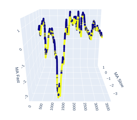
Fig 6: Visualizing the relationship between the moving averages and the target

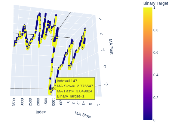
Fig 7: Our moving averages appear to cluster bullish and bearish price action to a reasonable extent

Let's see if maybe the volatility of the market has an effect on the target. We'll replace time from the x-axis and instead place the ATR value, and the slow and fast-moving averages will retain their positions.

# Create a 3D scatter plot showing the ineteraction between the slow and fast moving average and the ATR
fig = px.scatter_3d(
    data, x='ATR', y='MA Slow', z='MA Fast',
    color='Binary Target',
    title="3D Scatter Plot of ATR, The Slow Moving Average, and The Fast Moving Average",
    labels={'x': 'ATR', 'y': 'MA Fast', 'z':'MA Slow'}
)

# Update layout for custom size
fig.update_layout(
    width=800,  # Width of the figure in pixels
    height=600  # Height of the figure in pixels
)

# Adjust marker size for visibility
fig.update_traces(marker=dict(size=2))  # Set marker size to a smaller value

fig.show()

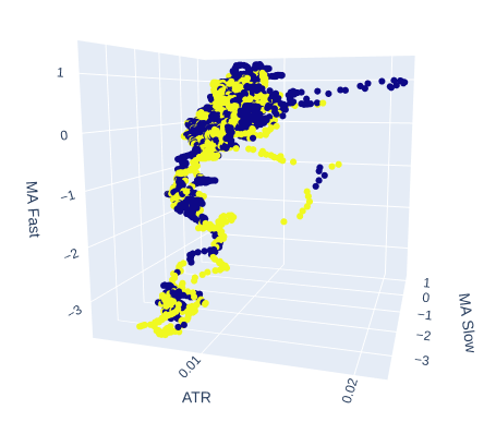
Fig 8: The ATR seems to add little clarity to our picture of the market. We may need to transform the volatility reading a little, for it to be informative

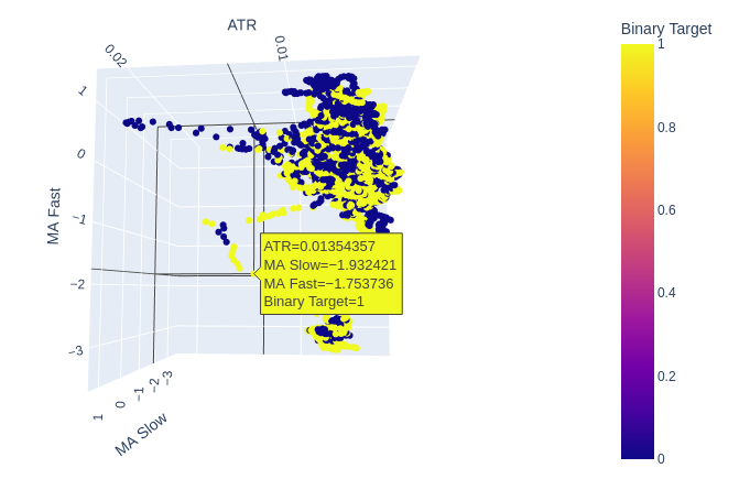
Fig 9: The ATR appears to expose clusters of bullish and bearish price action. However, the clusters are small, and may not occur frequently enough to be part of a reliable trading strategy

The 2 moving averages and the stochastic oscillator together give our market data a new structure all together.

# Creating a 3D scatter plot of the slow and fast moving average and the stochastic oscillator
fig = px.scatter_3d(
    data, x='MA Fast', y='MA Slow', z='Stoch Main',
    color='Binary Target',
    title="3D Scatter Plot of Time, Close Price, and The Stochastic Oscilator",
    labels={'x': 'Time', 'y': 'Close Price', 'z': 'Stochastic Oscilator'}
)

# Update layout for custom size
fig.update_layout(
    width=800,  # Width of the figure in pixels
    height=600  # Height of the figure in pixels
)

# Adjust marker size for visibility
fig.update_traces(marker=dict(size=2))  # Set marker size to a smaller value

fig.show()

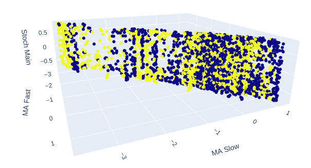
Fig 10:The Stochastic Main reading and the 2 moving averages give some well-defined bullish and bearish zones

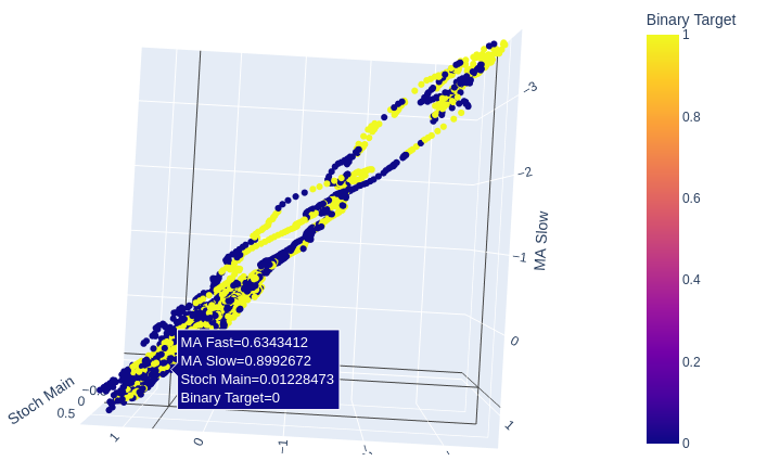
Fig 11: The relationship between the 2 moving averages and the stochastic may better suited for exposing bullish price action than bearish price action

Given that we are using 3 technical indicators and 4 different price quotes, our data has 7 dimensions, but we can only visualize 3 at most. We can transform our data into just 2 columns using dimensionality reduction techniques. Principal Components Analysis is a popular choice for solving these kinds of problems. We can use the algorithm to summarize all the columns in our original data set into just 2 columns.

We'll then create a scatter plot of the 2 principal components and determine how well they expose the target for us.

# Selecting features to include in PCA
features = data[['Open', 'High', 'Low', 'Close', 'MA Fast', 'MA Slow']]
pca = PCA(n_components=2)
pca_components = pca.fit_transform(features.dropna())

# Plotting PCA results
# Create a new DataFrame with PCA results and target variable for plotting
pca_df = pd.DataFrame(data=pca_components, columns=['PC1', 'PC2'])
pca_df['target'] = data['Binary Target'].iloc[:len(pca_components)]  # Add target column

# Plot PCA results with binary target as hue
fig = px.scatter(
    pca_df, x='PC1', y='PC2', color='target',
    title="2D PCA Plot of OHLC Data with Target Hue",
    labels={'PC1': 'Principal Component 1', 'PC2': 'Principal Component 2', 'color': 'Target'}
)

# Update layout for custom size
fig.update_layout(
    width=600,  # Width of the figure in pixels
    height=600  # Height of the figure in pixels
)

fig.show()

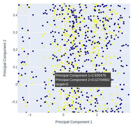
Fig 12: Zooming in on a random portion of our scatter plot of the first 2 principal components to see how well they separate price fluctuations

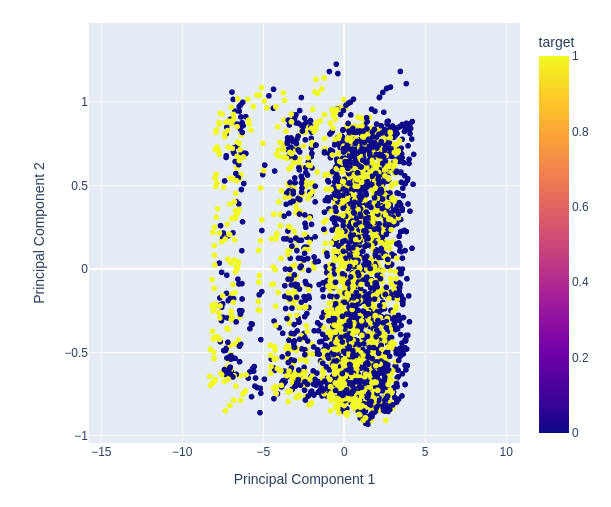
Fig 13:Visualizing our data shows us that PCA doesn't add better separation to the data set

Unsupervised learning algorithms like KMeansClustering may be able to learn patterns in the data not apparent to us. The algorithm will create labels for the data it is given, without any information about the target.

The idea is that, our KMeans clustering algorithm can learn 2 classes from our data set that will separate our 2 classes well. Unfortunately, the KMeans algorithm didn't really live up to our expectations. We observed both bullish and bearish price action across both classes, the algorithm generated from the data.

from sklearn.cluster import KMeans

# Select relevant features for clustering 
features = data[['Open', 'High', 'Low', 'Close', 'MA Fast', 'MA Slow','Stoch Main','ATR']]
target = data['Binary Target'].iloc[:len(features)]  # Ensure target matches length of features

# Apply K-means clustering with 2 clusters
kmeans = KMeans(n_clusters=2)
clusters = kmeans.fit_predict(features)

# Create a DataFrame for plotting with target and cluster labels
plot_data = pd.DataFrame({
    'target': target,
    'cluster': clusters
})

# Plot with seaborn's catplot to compare the binary target and cluster assignments
sns.catplot(x='cluster', hue='target',kind='count', data=plot_data)
plt.title("Comparison of K-means Clusters with Binary Target")
plt.show()

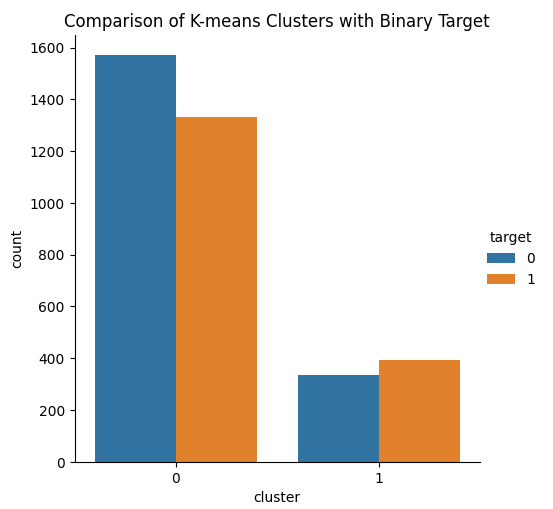
Fig 14: Visualizing the 2 clusters, our KMeans algorithm learned from the market data

We can also test for relationships between the variables by measuring the correlation of each input with our target. None of our inputs have strong correlation coefficients with our target. Please note, this does not disprove the existence of a relationship we can model.

#Read in the data
data = pd.read_csv("Market Data EURGBP MA Stoch ATR  As Series.csv")

#Add targets
data["ATR Target"] = data["ATR"].shift(-look_ahead)
data["Target"] = data["Close"].shift(-look_ahead) - data["Close"]

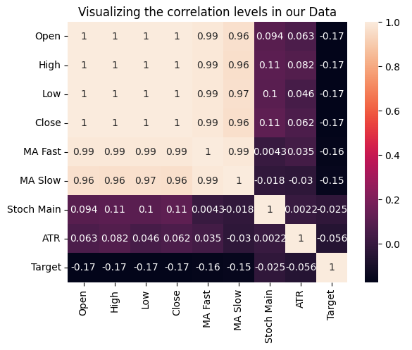
Fig 15: Visualizing the correlation levels in our dataset

Let us now transform our input data. We have 3 forms we can use our indicators in:

1. The current reading.
2. Markov states.
3. Difference between its past value.

Each form has its own set of advantages and disadvantages. The optimal form to present the data in will vary depending on factors such as which indicator is being modeled and which market the indicator is being applied on. Since there is no other way determining the ideal choice, we will perform a brute force search over all possible options for each indicator.

Pay attention to the "Time" column in our dataset. Note that our data runs from the year 2010 until 2021. This does not overlap with the period which will we use for our back test?

#Let's think of the different ways we can show the indicators to our AI Model
#We can describe the indicator by its current reading
#We can describe the indicator using markov states
#We can describe the change in the indicator's value

#Let's see which form helps our AI Model predict the future ATR value
data["ATR 1"] = 0
data["ATR 2"] = 0

#Set the states
data.loc[data["ATR"] > data["ATR"].shift(look_ahead),"ATR 1"] = 1
data.loc[data["ATR"] < data["ATR"].shift(look_ahead),"ATR 2"] = 1

#Set the change in the ATR
data["Change in ATR"] = data["ATR"] - data["ATR"].shift(look_ahead)

#We'll do the same for the stochastic
data["STO 1"] = 0
data["STO 2"] = 0
data["STO 3"] = 0

#Set the states
data.loc[data["Stoch Main"] > 80,"STO 1"] = 1
data.loc[data["Stoch Main"] < 20,"STO 2"] = 1
data.loc[(data["Stoch Main"] >= 20) & (data["Stoch Main"] <= 80) ,"STO 3"] = 1

#Set the change in the stochastic
data["Change in STO"] = data["Stoch Main"] - data["Stoch Main"].shift(look_ahead)

#Finally the moving averages
data["MA 1"] = 0
data["MA 2"] = 0

#Set the states
data.loc[data["MA Fast"] > data["MA Slow"],"MA 1"] = 1
data.loc[data["MA Fast"] < data["MA Slow"],"MA 2"] = 1

#Difference in the MA Height
data["Change in MA"] = (data["MA Fast"] - data["MA Slow"]) - (data["MA Fast"].shift(look_ahead) - data["MA Slow"].shift(look_ahead))

#Difference in price
data["Change in Close"] = data["Close"] - data["Close"].shift(look_ahead)

#Clean the data
data.dropna(inplace=True)
data.reset_index(inplace=True,drop=True)

#Drop the last 2 years of test data
data = data.iloc[:((-365*2) - 18),:]
data.dropna(inplace=True)
data.reset_index(inplace=True,drop=True)

data

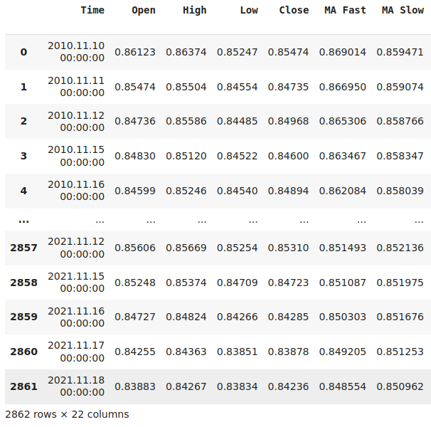
Fig 16: Visualizing our market data after transforming it accordingly

Let's see which form of presentation is most effective for our model to learn the change in price given the change in our indicators. We will use a gradient boosting regressor tree as our model of choice.

#Let's see which method of presentation is most effective
from sklearn.ensemble import GradientBoostingRegressor
from sklearn.linear_model import Ridge
from sklearn.model_selection import TimeSeriesSplit,cross_val_score

Define the parameters of our time series cross validation.

tscv = TimeSeriesSplit(n_splits=5,gap=look_ahead)

Now let us set a threshold. Any model that can be outperformed by simply using the Close price to predict the change in price, is not a good model.

#Our baseline accuracy forecasting the change in price using current price
np.mean(cross_val_score(GradientBoostingRegressor(),data.loc[:,["Close"]],data.loc[:,"Target"],cv=tscv))

-0.14861941262441164

On most problems, we can always perform better by using the change in price, as opposed to just the current price reading.

#Our accuracy forecasting the change in price using current change in price
np.mean(cross_val_score(GradientBoostingRegressor(),data.loc[:,["Change in Close"]],data.loc[:,"Target"],cv=tscv))

-0.1033528767401429

Our model can perform even better if we give it the stochastic oscillator instead.

#Our accuracy forecasting the change in price using the stochastic
np.mean(cross_val_score(GradientBoostingRegressor(),data.loc[:,["Stoch Main"]],data.loc[:,"Target"],cv=tscv))

-0.09152071417994265

However, is this the best we can do? What would happen if we gave our model, the change in the stochastic oscillator, instead? Our ability to forecast the changes in price gets better!

#Our accuracy forecasting the change in price using the stochastic
np.mean(cross_val_score(GradientBoostingRegressor(),data.loc[:,["Change in STO"]],data.loc[:,"Target"],cv=tscv))

-0.07090156075020868

What do you think will happen if we now perform our dummy encoding approach? We created 3 columns to simply tell us which state the indicator is in. Our error rates shrink. This result is very interesting, we are performing a lot better than a trader who is trying to predict changes in price given the current price or the current reading of the stochastic oscillator. But keep in mind, we do not know if this is true across all possible markets. We are only confident this is true on the EURGBP Market on the Daily Time Frame.

#Our accuracy forecasting the change in price using the stochastic
np.mean(cross_val_score(GradientBoostingRegressor(),data.loc[:,["STO 1","STO 2","STO 3"]],data.loc[:,"Target"],cv=tscv))

-0.016422009836789698

Let's now assess our accuracy predicting the changes in price using the current reading of the two moving averages. The results do not look good, our error rates are higher than our accuracy using just the Close price to predict the future change in price. This model should be abandoned and is not fit for use in production.

#Our accuracy forecasting the change in price using the moving averages
np.mean(cross_val_score(GradientBoostingRegressor(),data.loc[:,["MA Slow","MA Fast"]],data.loc[:,"Target"],cv=tscv))

-0.41868715470139356

If we transform our data so that we can see the change in the moving average values, our results get better. However, we will still be better off using a simpler model that just takes the current close price.

#Our accuracy forecasting the change in price using the change in the moving averages
np.mean(cross_val_score(GradientBoostingRegressor(),data.loc[:,["Change in MA"]],data.loc[:,"Target"],cv=tscv))

-0.11570348378760871

However, if we apply our dummy encoding technique to the market data, we start to outperform any trader in the same market using ordinary price quotes on the Daily Timeframe. Our error rates shrink to new lows we had not seen before. This transformation is powerful. Recall that it helps the model focus more on the critical changes in the value of the indicator, as opposed to learning the exact mapping of each possible value our indicator can take.

#Our accuracy forecasting the change in price using the state of moving averages
np.mean(cross_val_score(GradientBoostingRegressor(),data.loc[:,["MA 1","MA 2"]],data.loc[:,"Target"],cv=tscv))

-0.013366216034961066

For readers who are learning this topic for the first time, this section is particularly important. As human beings, we tend to see patterns, even when they do not exist. What you have read so far may leave you with the impression that dummy encoding is always your best friend. However, this is not the case. Observe what happens as we try to optimize our final AI model that is going to predict the future ATR reading.

Do not compare the results you will see now, with the results we have just discussed. The units of the target have changed. Therefore, a direct comparison between our accuracy predicting the changes in price and our accuracy predicting the future ATR value makes no sense practically.

We are essentially creating a new threshold. Our accuracy of predicting the ATR using previous ATR values is our new baseline. Any technique that results in greater error is not optimal and should be abandoned.

#Our accuracy forecasting the ATR
np.mean(cross_val_score(GradientBoostingRegressor(),data.loc[:,["ATR"]],data.loc[:,"ATR Target"],cv=tscv))

-0.023953677440629772

So far, today, we observed that our error rates decreased whenever we passed our model the difference in the data as opposed to the data in its current form. However, this time around, our error got worse.

#Our accuracy forecasting the ATR using the change in the ATR
np.mean(cross_val_score(GradientBoostingRegressor(),data.loc[:,["Change in ATR"]],data.loc[:,"ATR Target"],cv=tscv))

-0.5916640039518372

Additionally, we dummy encoded the ATR indicator to denote if it had been rising or falling. Our error rates were still unacceptable. Therefore, we will use our ATR indicator as it is and the Stochastic Oscillator and Our Moving Averages will be dummy encoded.

#Our accuracy forecasting the ATR using the current state of the ATR
np.mean(cross_val_score(GradientBoostingRegressor(),data.loc[:,["ATR 1","ATR 2"]],data.loc[:,"ATR Target"],cv=tscv))

-0.49362780061515144

Exporting To ONNX

Open Neural Network Exchange (ONNX) is an open-source protocol that defines a universal representation for all machine learning models. This allows us to develop and share models in any language as long as that language fully extends support to the ONNX API. ONNX allows us to export the AI models we have just developed and use them directly in our AI models to make our trading decisions, as opposed to used fixed trading rules.

#Load the libraries we need
import onnx
from   skl2onnx import convert_sklearn
from   skl2onnx.common.data_types import FloatTensorType

Define the input shape of each model.

#Define the input shapes
#ATR AI
initial_types_atr = [('float_input', FloatTensorType([1, 1]))]
#MA AI
initial_types_ma  = [('float_input', FloatTensorType([1, 2]))]
#STO AI
initial_types_sto = [('float_input', FloatTensorType([1, 3]))]

Fit each model on all the data we have.

#ATR AI Model
atr_ai = GradientBoostingRegressor().fit(data.loc[:,["ATR"]],data.loc[:,"ATR Target"])
#MA AI Model
ma_ai = GradientBoostingRegressor().fit(data.loc[:,["MA 1","MA 2"]],data.loc[:,"Target"])
#Stochastic AI Model
sto_ai = GradientBoostingRegressor().fit(data.loc[:,["STO 1","STO 2","STO 3"]],data.loc[:,"Target"])

Save the ONNX models.

#Save the ONNX models
onnx.save(convert_sklearn(atr_ai, initial_types=initial_types_atr),"EURGBP ATR.onnx")
onnx.save(convert_sklearn(ma_ai, initial_types=initial_types_ma),"EURGBP MA.onnx")
onnx.save(convert_sklearn(sto_ai, initial_types=initial_types_sto),"EURGBP Stoch.onnx")

Implementing in MQL5

We will use the same trading algorithm we have developed thus far. We will only change the fixed rules we initially gave, and instead allow our trading application to place its trades whenever our models give us a clear signal. Furthermore, we will start by importing the ONNX Models we have developed.

//+------------------------------------------------------------------+
//|                                         EURGBP Stochastic AI.mq5 |
//|                                        Gamuchirai Zororo Ndawana |
//|                          https://www.mql5.com/en/gamuchiraindawa |
//+------------------------------------------------------------------+
#property copyright "Gamuchirai Zororo Ndawana"
#property link      "https://www.mql5.com/en/gamuchiraindawa"
#property version   "1.00"

//+------------------------------------------------------------------+
//| Load the AI Modules                                              |
//+------------------------------------------------------------------+
#resource "\\Files\\EURGBP MA.onnx" as  const uchar ma_onnx_buffer[];
#resource "\\Files\\EURGBP ATR.onnx" as  const uchar atr_onnx_buffer[];
#resource "\\Files\\EURGBP Stoch.onnx" as  const uchar stoch_onnx_buffer[];

Now, define global variables that will store our model's forecasts.

//+------------------------------------------------------------------+
//| Global variables                                                 |
//+------------------------------------------------------------------+
double vol,bid,ask;
long atr_model,ma_model,stoch_model;
vectorf atr_forecast = vectorf::Zeros(1),ma_forecast = vectorf::Zeros(1),stoch_forecast = vectorf::Zeros(1);

We also need to update our deinitialization procedure. Our model should also release the resources that were being used by our ONNX models.

//+------------------------------------------------------------------+
//| Expert deinitialization function                                 |
//+------------------------------------------------------------------+
void OnDeinit(const int reason)
  {
//---
   IndicatorRelease(fast_ma_handler);
   IndicatorRelease(slow_ma_handler);
   IndicatorRelease(atr_handler);
   IndicatorRelease(stochastic_handler);
   OnnxRelease(atr_model);
   OnnxRelease(ma_model);
   OnnxRelease(stoch_model);
  }

Getting predictions from our ONNX models is not as expensive as training the models. However, to quickly back-test our trading algorithms, getting an AI prediction on every tick becomes expensive. Our back-tests will be a lot faster if we fetch predictions from our AI models every 5 minutes instead.

//+------------------------------------------------------------------+
//| Expert tick function                                             |
//+------------------------------------------------------------------+
void OnTick()
  {
//--- Fetch updated quotes
   update();

//--- Only on new candles
   static datetime time_stamp;
   datetime current_time = iTime(_Symbol,PERIOD_M5,0);
   if(time_stamp != current_time)
     {
      time_stamp = current_time;
      //--- If we have no open positions, check for a setup
      if(PositionsTotal() == 0)
        {
         find_setup();
        }
     }
  }

We also need to update the function responsible for setting up our technical indicators. The function will set up our AI models and validate the models have been loaded correctly.

//+------------------------------------------------------------------+
//| Setup technical market data                                      |
//+------------------------------------------------------------------+
void setup(void)
  {
//--- Setup our indicators
   slow_ma_handler    = iMA("EURGBP",PERIOD_D1,slow_period,0,MODE_EMA,PRICE_CLOSE);
   fast_ma_handler    = iMA("EURGBP",PERIOD_D1,fast_period,0,MODE_EMA,PRICE_CLOSE);
   stochastic_handler = iStochastic("EURGBP",PERIOD_D1,5,3,3,MODE_EMA,STO_CLOSECLOSE);
   atr_handler        = iATR("EURGBP",PERIOD_D1,atr_period);
//--- Fetch market data
   vol = lot_multiple * SymbolInfoDouble("EURGBP",SYMBOL_VOLUME_MIN);

//--- Create our onnx models
   atr_model   = OnnxCreateFromBuffer(atr_onnx_buffer,ONNX_DEFAULT);
   ma_model    = OnnxCreateFromBuffer(ma_onnx_buffer,ONNX_DEFAULT);
   stoch_model = OnnxCreateFromBuffer(stoch_onnx_buffer,ONNX_DEFAULT);

//--- Validate our models
   if(atr_model == INVALID_HANDLE || ma_model == INVALID_HANDLE || stoch_model == INVALID_HANDLE)
     {
      Comment("[ERROR] Failed to load AI modules: ",GetLastError());
     }

//--- Set the sizes of our ONNX models
   ulong atr_input_shape[]  = {1,1};
   ulong ma_input_shape[]   = {1,2};
   ulong sto_input_shape[]  = {1,3};

   if(!(OnnxSetInputShape(atr_model,0,atr_input_shape)) || !(OnnxSetInputShape(ma_model,0,ma_input_shape)) || !(OnnxSetInputShape(stoch_model,0,sto_input_shape)))
     {
      Comment("[ERROR] Failed to load AI modules: ",GetLastError());
     }

   ulong output_shape[] = {1,1};

   if(!(OnnxSetOutputShape(atr_model,0,output_shape)) || !(OnnxSetOutputShape(ma_model,0,output_shape)) || !(OnnxSetOutputShape(stoch_model,0,output_shape)))
     {
      Comment("[ERROR] Failed to load AI modules: ",GetLastError());
     }
  }

In our previous trading algorithm we simply opened our positions so long the indicators aligned for us. Now, we will instead open our positions if our AI models give us a clear trading signal. Additionally, our take profit and stop loss levels will be dynamically set to anticipated volatility levels. Hopefully, we have created a filter using AI that will give us more profitable trading signals.

//+------------------------------------------------------------------+
//| Check if we have an oppurtunity to trade                         |
//+------------------------------------------------------------------+
void find_setup(void)
  {
//--- Predict future ATR values
   vectorf atr_model_input = vectorf::Zeros(1);
   atr_model_input[0] = (float) atr[0];

//--- Predicting future price using the stochastic oscilator
   vectorf sto_model_input = vectorf::Zeros(3);

   if(stochastic[0] > 80)
     {
      sto_model_input[0] = 1;
      sto_model_input[1] = 0;
      sto_model_input[2] = 0;
     }

   else
      if(stochastic[0] < 20)
        {
         sto_model_input[0] = 0;
         sto_model_input[1] = 1;
         sto_model_input[2] = 0;
        }

      else
        {
         sto_model_input[0] = 0;
         sto_model_input[1] = 0;
         sto_model_input[2] = 1;
        }

//--- Finally prepare the moving average forecast
   vectorf ma_inputs = vectorf::Zeros(2);
   if(fast_ma[0] > slow_ma[0])
     {
      ma_inputs[0] = 1;
      ma_inputs[1] = 0;
     }

   else
     {
      ma_inputs[0] = 0;
      ma_inputs[1] = 1;
     }

   OnnxRun(stoch_model,ONNX_DEFAULT,sto_model_input,stoch_forecast);
   OnnxRun(atr_model,ONNX_DEFAULT,atr_model_input,atr_forecast);
   OnnxRun(ma_model,ONNX_DEFAULT,ma_inputs,ma_forecast);

   Comment("ATR Forecast: ",atr_forecast[0],"\nStochastic Forecast: ",stoch_forecast[0],"\nMA Forecast: ",ma_forecast[0]);

//--- Can we buy?
   if((ma_forecast[0] > 0) && (stoch_forecast[0] > 0))
     {
      Trade.Buy(vol,"EURGBP",ask,(ask - (atr[0] * atr_multiple)),(ask + (atr_forecast[0] * atr_multiple)),"EURGBP");
     }

//--- Can we sell?
   if((ma_forecast[0] < 0) && (stoch_forecast[0] < 0))
     {
      Trade.Sell(vol,"EURGBP",bid,(bid + (atr[0] * atr_multiple)),(bid - (atr_forecast[0] * atr_multiple)),"EURGBP");
     }
  }
//+------------------------------------------------------------------+

We will perform our back test over the same period we used before, from the beginning of January 2022 until June 2024. Recall that when we were training our AI model, we did not have any data in the range of the back test. We will test using the same symbol, the EURGBP pair on the same time frame, the Daily Time frame.

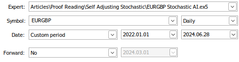
Fig 17: Back testing our AI model

We will fix all other parameters of the back test so that our tests are essentially identical. We are essentially trying to isolate the difference made by having our decisions being made by our AI Models.

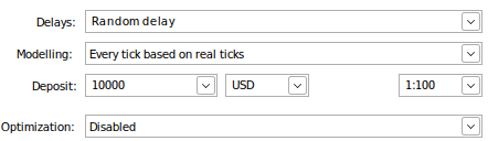
Fig 18: The remaining parameters of our back test

Our trading strategy was more profitable over the test period! This is great news because the models were not shown the data we are using in the back test. Therefore, we can have positive expectations when using this model to trade a real account.

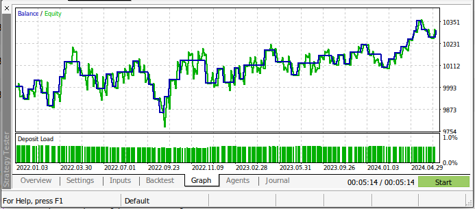
Fig 19: The results of back-testing our AI model over the test dates

The new model placed fewer trades over the back test, but it had a higher proportion of winning trades than our old trading algorithm. Additionally, our Sharpe Ratio is now positive and only 44% of our trades were losing trades.

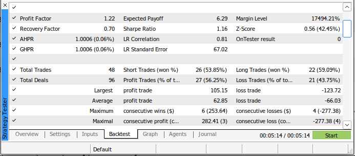
Fig 20: Detailed results from back testing our AI-powered trading strategy

Conclusion

Hopefully, after reading this article, you will agree with me that AI can genuinely be used to improve our trading strategies. Even the oldest classical trading strategy can be reimagined using AI, and revamped to new levels of performance. It appears the trick lies in intelligently transforming your indicator data to help the models learn effectively. The dummy encoding technique we demonstrated today has helped us a lot. But we cannot conclude it is the best choice to make across all possible markets. It is possible that the dummy encoding technique may be the best choice we have for a certain group of markets. However, we can confidently conclude that the moving averages cross-over can effectively be revamped using AI.