Deep Learning GRU model with Python to ONNX with EA, and GRU vs LSTM models

Introduction

This is the continuation of Deep Learning Forecast and Order Placement using Python, the MetaTrader5 Python package and an ONNX model file, but you continue this one without the previous one. All will be explained. Everything we will use is included in this article. In this section, we will guide you through the entire process, culminating in the creation of an Expert Advisor (EA) for trading and subsequent testing.

Machine learning is a subset of artificial intelligence (AI) that focuses on developing algorithms and statistical models that enable computers to perform tasks without being explicitly programmed. The primary goal of machine learning is to enable computers to learn from data and improve their performance over time.

How models work

Let use of the basic principles underlying the operation and application of machine learning models. While this may seem elementary to those who already have experience with statistical modeling or machine learning, rest assured that we will quickly move on to developing sophisticated and robust models.

We will initially focus on a model known as a decision tree. While there are more complicated models that offer higher predictive accuracy, decision trees serve as an accessible entry point due to their simplicity and fundamental role in constructing some of the most advanced models in the field of data science.

To simplify things, let us start with the most rudimentary form of a decision tree.

Here we categorizes houses into only two different groups. The expected price for each eligible house is derived from the historical average price of houses within the same category.

It uses data to determine the optimal method for categorizing homes into these two groups and then determines the expected price for each group. This crucial step, in which the model captures patterns from the data, is known as fitting or training the model. The data set used for this purpose is called the training data.

The intricacies of model fitting, including data segmentation decisions, are sufficiently complex and will be covered in more detail later. Once the model has been fitted, it can be applied to new data to forecast prices for additional homes.

Improving the decision tree

Which of the two decision trees shown below is more likely to emerge from the process of adjusting the training data for real estate?

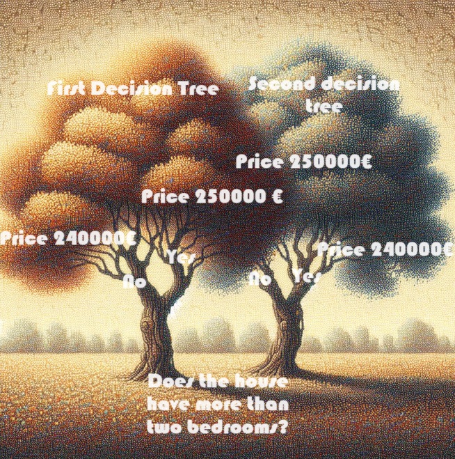
The decision tree on the left (decision tree 1) is probably more in line with reality, as it reflects the correlation between the number of bedrooms and higher house sales prices. However, its main drawback is that it does not take into account many other factors that affect house prices, such as the number of bathrooms, plot size, location, etc.

To account for a wider range of factors, one can use a tree with additional "splits" called a "deeper" tree. For example, a decision tree that takes into account the total lot size of each home might look like this:

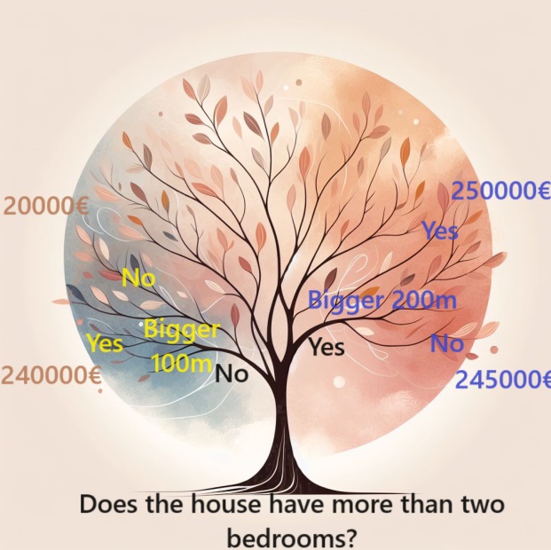
To estimate the price of a house, follow the branches of the decision tree, always choosing the path that matches the specific characteristics of the house. The predicted price for the house is at the end of the tree. This particular point where a prediction is made is called a "leaf"

The divisions and values at these leaves are influenced by the data, prompting you to look at the data set you are working with.

Using Pandas for data

In the initial phase of any machine learning project, you need to familiarize yourself with the data set. This is where the Pandas library proves to be indispensable. Data scientists typically use Pandas as their primary tool for examining and processing data. In code, it is usually abbreviated as "pd"

import pandas as pd

Selecting data for modeling

The data set has an overwhelming number of variables that make it difficult to understand or even present clearly. How can we organize this vast amount of data into a more manageable form to better understand it?

Our first approach is to select a subset of variables based on intuition. On forwards, we will introduce statistical techniques that enable automatic prioritization of the variables.

To identify the variables or columns to be selected, we first need to examine a comprehensive list of all columns in the dataset.

We imported this data, from with this:

mt5.copy_rates_range("EURUSD", mt5.TIMEFRAME_H1, start_date, end_date)

Building your model

For creating your models, the best resource for you is the scikit-learn library, often abbreviated as sklearn in the code. Scikit-learn is the preferred choice for modeling the types of data typically stored in DataFrames.

Here are the key steps in creating and using a model:

• Define: Determine the type of model you want to create. Is it a decision tree, or will you choose a different model? You also define specific parameters for the selected model type.
• Customize:This phase is the core of modeling, where your model learns and captures patterns from the data provided. It involves training the model on your data set.
• Predict:As simple as it sounds, this step is where your trained model is used to make predictions on new or unseen data. The model generalizes what it has learned to make educated predictions.
• Evaluate:Evaluate the accuracy of your model's predictions. This crucial step compares the output of the model with the actual results so you can assess its performance and reliability.

Using scikit-learn, these steps provide a structured framework for efficiently building, training and evaluating models tailored to the different data typically found in DataFrames.

The gated recurrent unit (GRU)

Wikipedia say's :

Gated recurrent units (GRUs) are a gating mechanism in recurrent neural networks, introduced in 2014 by Kyunghyun Cho.The GRU is like a long short-term memory (LSTM) with a gating mechanism to input or forget certain features, but lacks a context vector or output gate, resulting in fewer parameters than LSTM. GRU's performance on certain tasks of polyphonic music modeling, speech signal modeling and natural language processing was found to be similar to that of LSTM. GRUs showed that gating is indeed helpful in general, and Bengio's team came to no concrete conclusion on which of the two gating units was better.

GRU, an acronym for Gated Recurrent Unit, represents a variant of recurrent neural network (RNN) architecture akin to LSTM (Long Short-Term Memory).

Much like LSTM, GRU is crafted for modeling sequential data, enabling selective retention or omission of information across time. Notably, GRU boasts a streamlined architecture relative to LSTM, featuring fewer parameters. This characteristic enhances ease of training and computational efficiency.

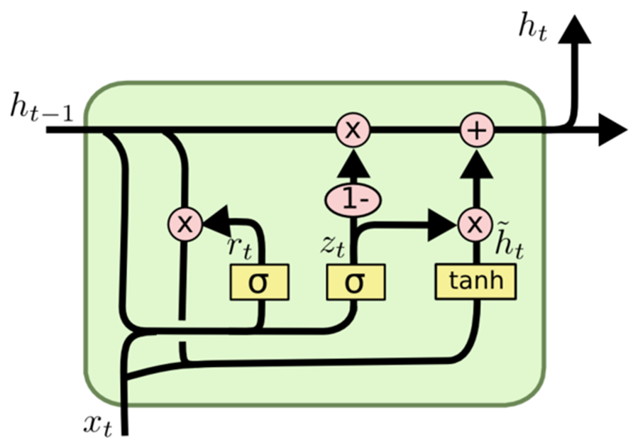
The primary distinction between GRU and LSTM lies in their handling of the memory cell state. In LSTM, the memory cell state is distinct from the hidden state and undergoes updates through three gates: the input gate, output gate, and forget gate. Conversely, GRU replaces the memory cell state with a "candidate activation vector," updated via two gates: the reset gate and update gate.

In summary, GRU emerges as a favored alternative to LSTM for sequential data modeling, particularly in scenarios where computational constraints exist or a simpler architecture is preferred.

How GRU Operates:

Similar to other recurrent neural network architectures, GRU processes sequential data element by element, adjusting its hidden state based on the current input and the preceding hidden state. At each time step, GRU calculates a "candidate activation vector" amalgamating information from the input and the previous hidden state. This vector then updates the hidden state for the subsequent time step.

The candidate activation vector is computed using two gates: the reset gate and the update gate. The reset gate determines the degree of forgetting from the prior hidden state, while the update gate influences the integration of the candidate activation vector into the new hidden state.

This is the model (GRU) we will choose for this article.

model.add(Dense(128, activation='relu', input_shape=(inp_history_size,1), kernel_regularizer=l2(k_reg)))
model.add(Dropout(0.05))
model.add(Dense(256, activation='relu', kernel_regularizer=l2(k_reg)))
model.add(Dropout(0.05))
model.add(Dense(128, activation='relu', kernel_regularizer=l2(k_reg)))
model.add(Dropout(0.05))
model.add(Dense(64, activation='relu', kernel_regularizer=l2(k_reg)))
model.add(Dropout(0.05))
model.add(Dense(1, activation='linear'))

First, we select the input in features and the target variable

if 'Close' in data.columns:
    data['target'] = data['Close']
else:
    data['target'] = data.iloc[:, 0]

# Extract OHLC columns
x_features = data[[0]]
# Target variable
y_target = data['target']

We run the data into training and testing sets

x_train, x_test, y_train, y_test = train_test_split(x_features, y_target, test_size=0.2, shuffle=False)

Here the test size is a 20 %, usually, tests sizes are chosen to be less than 30% (to not overfit)

Sequential Model Initialization:

model = Sequential()

This line creates an empty sequential model, which allows you to add layers in a step-by-step fashion.

Adding Dense Layers:

model.add(Dense(128, activation='relu', input_shape=(X_train.shape[1],), kernel_regularizer=l2(k_reg)))
model.add(Dense(256, activation='relu', kernel_regularizer=l2(k_reg)))
model.add(Dense(128, activation='relu', kernel_regularizer=l2(k_reg)))
model.add(Dense(64, activation='relu', kernel_regularizer=l2(k_reg)))

The dense layer is a fully connected layer in a neural network.

The numbers in the brackets indicate the number of neurons in each layer. The first layer therefore consists of 128 neurons, the second of 256, the third of 128 and the fourth of 64.

The activation function 'relu' (Rectified Linear Unit) is used to introduce a non-linearity after each layer, which helps the model to learn complex patterns.

The parameter input_shape is only specified in the first layer and defines the shape of the input data. In this case, it corresponds to the number of features in the input data.

kernel_regularizer=l2(k_reg) applies L2 regularization to the weights of the layer and helps to prevent overfitting by penalizing large weight values.

Output Layer:

model.add(Dense(1, activation='linear'))

• The last layer consists of a single neuron, which is typical for a regression task (prediction of a continuous value).
• The 'linear' activation function is used, which means that the output is a linear combination of the inputs without further transformation.
• To summarize, this model consists of several dense layers with rectified linear unit activation functions followed by a linear output layer. For regularization, L2 regularization is applied to the weights. This architecture is typically used for regression tasks where the goal is to predict a numerical value.

We now compile the model

# Compile the model[]
model.compile(optimizer='adam', loss='mean_squared_error')

Optimizer:

The optimizer is a crucial component of the training process. It determines how the weights of the model are updated during training to minimize the loss function. adam' is a popular optimization algorithm known for its efficiency in training neural networks. It adjusts the learning rates for each parameter individually and is therefore suitable for a wide range of problems.

Loss Function:

The loss parameter defines the target that the model tries to minimize during training. In this case, 'mean_squared_error' is used as the loss function. The mean squared error (MSE) is a common choice for regression problems where the goal is to minimize the mean squared difference between the predicted values and the actual values. It is suitable for problems where the output is a continuous value. MAE calculates the average of the absolute differences between the predicted values and the actual values.

All errors are treated with the same significance regardless of their direction. A lower MAE also means better model performance.

To summarize, the model.compile statement configures the neural network model for training. It specifies the optimizer ('adam') for updating the weights during training and the loss function ('mean_squared_error') that should minimize the model. This compilation step is a necessary preliminary stage for training the model with data.

And we train the previously defined neural network model.

# Train the model
model.fit(X_train_scaled, y_train, epochs=int(epoch), batch_size=256, validation_split=0.2, verbose=1)

Training data:

X_train_scaled : This is the input feature data for training, presumably scaled or preprocessed to ensure numerical stability.

y_train : These are the corresponding target values or labels for the training data.

Training configuration:

epochs=int(epoch) : This parameter specifies how many times the entire training data set is passed forward and backward through the neural network.

int(epoch) specifies that the number of epochs is determined by the variable epoch.

batch_size=256 : During each epoch, the training data is divided into batches, and the weights of the model are updated after each batch is processed. Here, each batch consists of 256 data points.

Validation data:

validation_split=0.2 : This parameter specifies that 20% of the training data is used as the validation set. The performance of the model on this set is monitored during training, but is not used for updating the weights.

Verbosity:
verbose=1 : This parameter controls the verbosity of the training output. A value of 1 means that the training progress is displayed in the console.

During the training process, the model learns to make predictions by adjusting its weights based on the provided input data ( X_train_scaled ) and target values ( y_train ). The validation split helps to evaluate the model's performance on unseen data and the training progress is displayed based on the verbosity setting.

Unveiling the Linear Unit

When we look at neuronal networks, we start with the basic building block: the individual neuron. Diagrammatically, a neuron, also known as a unit, looks like this when configured with a single input:

Unveiling the Linear Unit Mechanics

Let us explore the intricacies of the core component of a neural network: the single neuron. Visualized, a neuron with a single input x is represented as follows:

The input, labeled x, forms a connection to the neuron, and this connection has a weight, labeled w, attached to it. When information passes through this connection, the value is multiplied by the weight assigned to the connection. In the case of input x, what eventually reaches the neuron is the product w * x. By adjusting these weights, a neural network "learns" over time.

Now we introduce b, a special form of weighting called bias. Unlike other weights, bias has no input data associated with it. Instead, a value of 1 is inserted into the graph to ensure that the value that reaches the neuron is simply b (since 1 * b equals b). By introducing the bias, the neuron is enabled to change its output independently of its inputs.

Y = X*W + b*1

Embracing Multiple Inputs

And if we want to include more factors? Don't worry, because the solution is quite simple. By extending our model, we can seamlessly add additional input connections to the neuron, each corresponding to a specific feature.

To derive the output, we perform a straightforward process. Each input is multiplied by the appropriate connection weight and the results are lushly merged. The result is a holistic representation where the neuron skillfully processes multiple inputs, making the model more nuanced and reflecting the intricate interplay of different features. This method allows our neural network to capture a broader range of information, enhancing its ability to comprehensively recognise patterns.

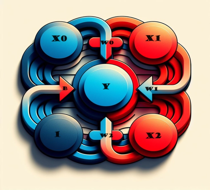
Expressed mathematically, the operation of this neuron is succinctly captured by the formula:

y = w 0 ⋅ x 0 + w 1 ⋅ x 1 + w 2 ⋅ x 2 + b =  y=w0​⋅x0​+w1​⋅x1​+w2​⋅x2​+b

In this equation:

• y represents the neuron's output.
• w 0 , w 1 , w 2 ​ denote the weights associated with the respective inputs x 0 , x 1 , x 2 ​.
• b stands for the bias term.

This linear unit, equipped with two inputs, possesses the capability to model a plane in a three-dimensional space. As the number of inputs surpasses two, the unit becomes adept at fitting hyperplanes—multi-dimensional surfaces that intricately capture the relationships between multiple input features. This flexibility allows the neural network to navigate and comprehend complex patterns in data that extend beyond simple linear relationships.

Linear Units in Keras

Crafting a neural network in Keras is seamlessly achieved through `keras.Sequential()`. This utility assembles a neural network by stacking layers, offering a straightforward approach to model creation. The layers encapsulate the essence of the network architecture, and among them, the `dense` layer becomes particularly pertinent for constructing models akin to those explored earlier.

model = Sequential()

In the forthcoming, we'll delve deeper into the intricacies of the dense layer, uncovering its capabilities and role in building robust and expressive neural network architectures.

Deep Neuronal Networks

Enhance the depth and expressive capacity of your network by integrating hidden layers. These concealed layers play a pivotal role in unraveling intricate relationships within the data, empowering your neural network to discern and capture complex patterns. Elevate your model's sophistication by strategically adding hidden layers, thereby enabling it to learn and represent nuanced features for more comprehensive and accurate predictions.

Exploring the Construction of Complex Neural Networks

We now embark on a journey to construct neural networks with the capability to grasp the intricate relationships that characterize deep neural networks' prowess.

Central to our approach is the concept of modularity—a strategy that involves piecing together a sophisticated network from elementary, functional units. Having previously delved into how a linear unit computes a linear function, our focus now shifts towards the fusion and adaptation of these individual units. By strategically combining and modifying these foundational components, we unlock the potential to model and understand more intricate and multifaceted relationships inherent in complex datasets. This serves as a gateway to crafting neural networks that can adeptly navigate and comprehend the nuanced patterns that define the realm of deep learning.

Layers Unveiled

In the intricate architecture of neural networks, neurons are systematically organized into layers. One noteworthy configuration that emerges is the dense layer—a consolidation of linear units sharing a common set of inputs.

This arrangement facilitates a powerful and interconnected structure, allowing neurons within the layer to collectively process and interpret information. As we delve into the intricacies of layers, the dense layer stands out as a foundational construct, illustrating how neurons can collaboratively contribute to the network's capacity to comprehend and learn complex relationships within the data.

 

Diverse Layers in Keras

In the realm of Keras, a "layer" encompasses a remarkably versatile entity. Essentially, it manifests as any form of data transformation. Numerous layers, exemplified by convolutional and recurrent layers, leverage neurons to metamorphose data, distinguished chiefly by the intricate patterns of connections they forge. Conversely, other layers serve purposes ranging from feature engineering to elementary arithmetic, showcasing the broad spectrum of transformations that can be orchestrated within the modular framework of a neural network. The diversity of layers underscores the adaptability and expansive capabilities that contribute to the rich tapestry of neural network architectures.

Empowering Neural Networks with Activation Functions

Surprisingly, the incorporation of two dense layers devoid of any intervening elements does not surpass the efficacy of a solitary dense layer. Dense layers in isolation confine us within the realm of linear structures, unable to transcend the boundaries of lines and planes. To break free from this linearity, we introduce a critical element: nonlinearity. This pivotal ingredient is embodied by activation functions.

Activation functions serve as the transformative force, injecting nonlinearity into the neural network. They provide the essential tool to navigate beyond linear constraints, allowing the model to discern intricate patterns and relationships within the data. In essence, activation functions are the catalysts that propel neural networks into realms of complexity, unlocking their capacity to capture the nuanced features inherent in diverse datasets.

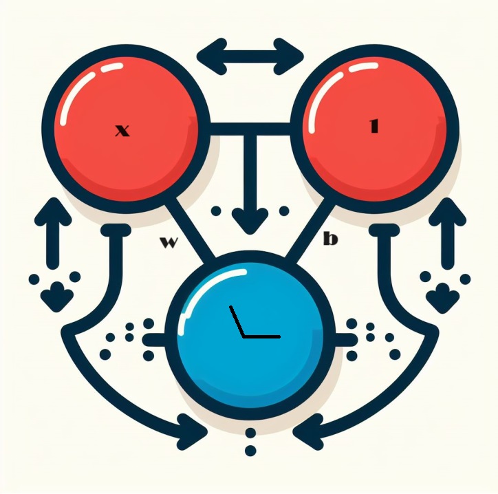
When we amalgamate the rectifier function with a linear unit, the result is a formidable entity known as a rectified linear unit or ReLU. In common parlance, the rectifier function is often referred to as the "ReLU function" for this reason. The application of ReLU activation to a linear unit transforms the output into max(0, w * x + b), a depiction that can be illustrated in a diagram as follows:

Strategic Layering with Dense Networks

Armed with newfound nonlinearity, let's explore the potency of layer stacking and how it enables us to orchestrate intricate data transformations.

Unveiling Hidden Layers in Neural Networks

Preceding the output layer, the layers in between are often dubbed "hidden layers" as their outputs remain concealed from direct observation.

Observe that the ultimate (output) layer adopts the guise of a linear unit, devoid of any activation function. This architectural choice aligns with tasks of regression nature, where the objective is to predict a numeric value. However, tasks such as classification might necessitate the incorporation of an activation function on the output layer to better suit the requirements of the specific task at hand.

Constructing Sequential Models

The Sequential model, as utilized thus far, seamlessly links a series of layers in a sequential manner—from the initial to the final layer. In this structural orchestration, the first layer serves as the recipient of the input, while the ultimate layer culminates in generating the coveted output. This sequential assembly mirrors the model depicted in the illustration above:

model = keras.Sequential([
    # the hidden ReLU layers
    layers.Dense(units=4, activation='relu', input_shape=[2]),
    layers.Dense(units=3, activation='relu'),
    # the linear output layer 
    layers.Dense(units=1),
])

Ensure cohesive layering by presenting all layers together within a list, akin to [layer, layer, layer, ...], as opposed to listing them separately. To seamlessly incorporate an activation function into a layer, simply specify its name within the activation argument. This streamlined approach ensures a concise and organized representation of your neural network architecture.

Selecting the Number of Units in a Dense Layer

The decision regarding the number of units in a layers.Dense layer (e.g., layers.Dense(units=4, ...) ) hinges on the unique characteristics of your problem and the intricacy of the patterns you aim to uncover in your data. Consider the following factors:

Problem Complexity:

• For simpler problems with less intricate relationships in the data, a smaller number of units, like 4, might be a suitable starting point.
• In more complex scenarios, characterized by nuanced and multifaceted relationships, opting for a larger number of units is often beneficial.

Data Size:

• Dataset size plays a role; larger datasets may accommodate a greater number of units for the model to learn from.
• Smaller datasets call for a more cautious approach to prevent overfitting and the potential of the model learning noise.

Model Capacity:

• The number of units influences the model's capacity to capture complex patterns, with an increase generally enhancing expressive power.
• Caution is advised to avoid over-parameterization, particularly when dealing with limited data, as it could lead to overfitting.

Experimentation:

• Experiment with different configurations, initiating with a modest number of units, training the model, and refining based on performance metrics and observations.
• Techniques like cross-validation provide insights into the model's generalization performance across various data subsets.

Remember, the choice of units is not universally fixed and may necessitate some trial and error. Monitoring the model's performance on a validation set and iteratively adjusting the architecture form a valuable part of the model development process.

We choose this:

model = Sequential()
model.add(Dense(128, activation='relu', input_shape=(X_train.shape[1],), kernel_regularizer=l2(k_reg)))
model.add(Dense(256, activation='relu', kernel_regularizer=l2(k_reg)))
model.add(Dense(128, activation='relu', kernel_regularizer=l2(k_reg)))
model.add(Dense(64, activation='relu', kernel_regularizer=l2(k_reg)))
model.add(Dense(1, activation='linear'))

First Layer (Input Layer):

Units (128): A relatively higher number of units, 128, in the first layer allows the model to capture diverse and complex patterns in the input data. This can be advantageous for extracting intricate features in the initial stages of the network. Activation ('relu'): The Rectified Linear Unit (ReLU) activation introduces nonlinearity, enabling the model to learn from complex relationships and patterns. Regularization (L2): The L2 regularization term ( kernel_regularizer=l2(k_reg) ) helps prevent overfitting by penalizing large weights in the layer.

Second and Third Layers:

Units (256 and 128): Maintaining a higher number of units in subsequent layers (256 and 128) continues to allow the model to capture and process complex information. The gradual reduction in the number of units helps create a hierarchy of features. Activation ('relu'): ReLU activation persists, promoting nonlinearity in each layer. Regularization (L2): Consistent application of L2 regularization across layers assists in preventing overfitting.

Fourth Layer: 

Units (64): A reduction in units further refines the representation of features, helping to distill essential information while maintaining a balance between complexity and simplicity. Activation ('relu'): ReLU activation endures, ensuring the preservation of nonlinear properties. Regularization (L2): The regularization term is consistently applied for stability.

Fifth Layer (Output Layer):

Units (1): The final layer with a single unit is well-suited for regression tasks where the goal is to predict a continuous numeric value. Activation ('linear'): The linear activation is appropriate for regression, allowing the model to directly output the predicted value without any additional transformation.

Overall, the chosen architecture seems tailored for a regression task, with a thoughtful balance between expressive capacity and regularization to prevent overfitting. The gradual reduction in the number of units facilitates the extraction of hierarchical features. This design suggests a comprehensive understanding of the complexity of the task and an effort to build a model that can generalize well to unseen data.

In summary, the gradual decrease in the number of units in the hidden layers, along with the specific choices for each layer, suggests a design aimed at capturing hierarchical and abstract representations of the input data. The architecture appears to balance model complexity with the need to avoid overfitting, and the choice of units aligns with the nature of the regression task at hand. The specific numbers might have been determined through experimentation and tuning based on the performance of the model on validation data.

Compile model

# Compile the model[]
model.compile(optimizer='adam', loss='mean_squared_error')

We have already delved into constructing fully-connected networks using stacks of dense layers. At the initial stage of creation, the network's weights are randomly set, signifying that the network lacks any prior knowledge. Now, our focus shifts to the process of training a neural network, unraveling the essence of how these networks learn.

As is customary in machine learning endeavors, we commence with a curated set of training data. Each example within this dataset comprises features (inputs) alongside an anticipated target (output). The crux of training the network lies in adjusting its weights to proficiently transform the input features into accurate predictions for the target output.

The triumphant training of a network for such a task implies that its weights encapsulate, to some extent, the relationship between these features and the target, as manifested in the training data.

Beyond the training data, two critical components come into play:

1. A "loss function" that gauges the efficacy of the network's predictions.
2. An "optimizer" tasked with instructing the network on how to iteratively adjust its weights for enhanced performance.

As we venture further into the training process, understanding the intricacies of these components becomes pivotal in nurturing a neural network's capacity to generalize and make accurate predictions on unseen data.

The Loss Function

While we've covered the architectural design of a network, the crucial aspect of instructing a network about the specific problem it should tackle is yet to be explored. This responsibility falls upon the loss function.

In essence, the loss function quantifies the difference between the true value of the target and the value predicted by the model. It serves as the yardstick for evaluating how effectively the model aligns its predictions with the actual outcomes.

A frequently used loss function in regression problems is the mean absolute error (MAE). In the context of each prediction, denoted as y_pred, the MAE assesses the difference from the true target, y_true, by calculating the absolute difference, abs(y_true - y_pred).

The cumulative MAE loss across a dataset is computed as the mean of all these absolute differences. This metric provides a comprehensive measure of the average magnitude of the prediction errors, guiding the model towards minimizing the overall discrepancy between its predictions and the true targets.

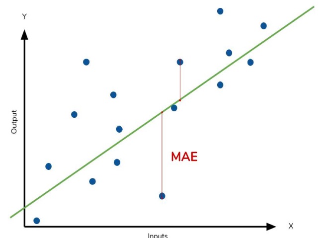
The mean absolute error represents the average distance between the fitted curve and the actual data points.

In addition to MAE, alternative loss functions commonly encountered in regression problems include mean-squared error (MSE) and the Huber loss, both of which are accessible in Keras.

Throughout the training process, the model relies on the loss function as a navigational guide to determine the optimal values for its weights—aiming for the lowest possible loss. In essence, the loss function communicates the network's objective, guiding it towards learning and refining its parameters to enhance predictive accuracy.

The Optimizer - Stochastic Gradient Descent

Having defined the problem the network is tasked to solve, the next crucial step is outlining how to solve it. This responsibility is shouldered by the optimizer—an algorithm dedicated to fine-tuning the weights with the objective of minimizing the loss.

In the realm of deep learning, the majority of optimization algorithms fall under the umbrella of stochastic gradient descent. These are iterative algorithms that train a network incrementally. Each training step follows this sequence:

1. Sample some training data and input it into the network to generate predictions.
2. Evaluate the loss by comparing the predictions against the true values.
3. Adjust the weights in a direction that reduces the loss.

This process is repeated iteratively until the desired level of loss reduction is achieved, or until further reduction becomes impractical. Essentially, the optimizer guides the network through the intricacies of weight adjustments, steering it towards the configuration that minimizes the loss and enhances predictive accuracy.

Each set of training data sampled in each iteration is termed a minibatch, often simply referred to as a "batch." On the other hand, a full sweep through the training data is known as an epoch. The number of epochs specified determines how many times the network processes each training example.

Learning Rate and Batch Size

The line undergoes only a modest shift in the direction of each batch rather than a complete overhaul. The magnitude of these shifts is governed by the learning rate. A smaller learning rate implies that the network requires exposure to more minibatches before its weights settle into their optimal values.

The learning rate and the size of the minibatches stand as the two paramount parameters influencing the trajectory of SGD training. Navigating their interplay can be nuanced, and the optimal selection isn't always apparent.

Thankfully, for most tasks, an exhaustive search for optimal hyperparameters isn't imperative for satisfactory outcomes. Adam, an SGD algorithm with an adaptive learning rate, eliminates the need for extensive parameter tuning. Its self-tuning nature renders it an excellent all-purpose optimizer suitable for a wide array of problems.

For this example we choosed ADAM as SGD and MSE as loss.

model.compile(optimizer='adam', loss='mean_squared_error')

When fitting,

# Train the model
model.fit(X_train_scaled, y_train, epochs=int(epoch), batch_size=256, validation_split=0.2, verbose=1)

we will see something like this:

44241/44241 [==============================] - 247s 6ms/step - loss: 0.0021 - val_loss: 8.0975e-04
Epoch 2/30
44241/44241 [==============================] - 247s 6ms/step - loss: 2.3062e-04 - val_loss: 0.0010
Epoch 3/30
44241/44241 [==============================] - 288s 7ms/step - loss: 2.3019e-04 - val_loss: 8.5903e-04
Epoch 4/30
44241/44241 [==============================] - 248s 6ms/step - loss: 2.3003e-04 - val_loss: 7.6378e-04
Epoch 5/30
44241/44241 [==============================] - 257s 6ms/step - loss: 2.2993e-04 - val_loss: 9.5630e-04
Epoch 6/30
44241/44241 [==============================] - 247s 6ms/step - loss: 2.2988e-04 - val_loss: 7.3110e-04
Epoch 7/30
44241/44241 [==============================] - 224s 5ms/step - loss: 2.2985e-04 - val_loss: 8.7191e-04

Overfitting and Underfitting

Keras maintains a record of the training and validation loss throughout the epochs while the model is being trained. We will delve into interpreting these learning curves and explore how to leverage them to enhance model development. Specifically, we will analyze the learning curves to identify signs of underfitting and overfitting, and explore a few strategies to address these issues.

Interpreting Learning Curves:

When considering information in the training data, it can be categorized into two components: signal and noise. The signal represents the part that generalizes, aiding our model in making predictions on new data. On the other hand, noise comprises random fluctuations stemming from real-world data and non-informative patterns that don't contribute to the model's predictive capabilities. Identifying and understanding this distinction is crucial.

During model training, we aim to select weights or parameters that minimize the loss on a training set. However, for a comprehensive evaluation of a model's performance, it is imperative to assess it on a new set of data – the validation data.

Effectively interpreting these curves (when plotting them) is essential for training deep learning models successfully.

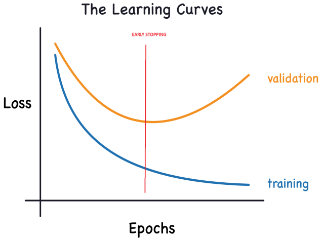
Now, the training loss decreases when the model acquires either signal or noise. However, the validation loss decreases only when the model learns signal, as any noise acquired from the training set fails to generalize to new data. Consequently, when the model learns signal, both curves exhibit a decline, while learning noise creates a gap between them. The magnitude of this gap indicates the extent of noise the model has acquired.

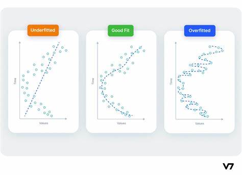
In an ideal scenario, we would aim to build models that learn all signal and none of the noise. However, achieving this ideal state is practically improbable. Instead, we navigate a trade-off. We can encourage the model to learn more signal at the expense of acquiring more noise. As long as this trade-off favors us, the validation loss will continue to decrease. Nevertheless, there comes a point where the trade-off becomes unfavorable, the cost outweighs the benefit, and the validation loss starts to increase.

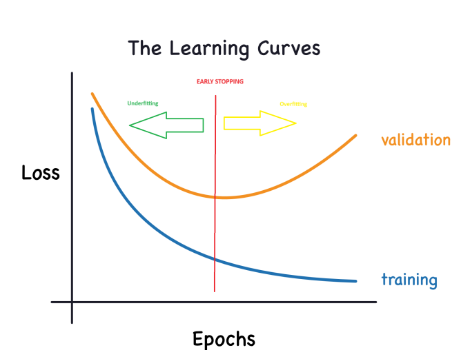
This trade-off highlights two potential challenges in model training: insufficient signal or excessive noise. Underfitting the training set occurs when the loss isn't minimized because the model hasn't learned enough signal. On the other hand, overfitting the training set happens when the loss isn't minimized because the model has absorbed too much noise. The key to training deep learning models lies in discovering the optimal balance between these two scenarios.

The other graph will now look like this:

Model Capacity:

A model's capacity denotes its ability to grasp and comprehend intricate patterns. In the context of neural networks, this is predominantly influenced by the number of neurons and their interconnectedness. If it seems that your network is inadequately capturing the complexity of the data (underfitting), consider enhancing its capacity.

The capacity of a network can be increased by either broadening it (adding more units to existing layers) or deepening it (incorporating more layers). Wider networks excel at learning more linear relationships, whereas deeper networks are inclined towards capturing more nonlinear patterns. The choice between the two depends on the nature of the dataset.

Early Stopping:

As previously discussed, when a model is excessively incorporating noise during training, the validation loss might begin to rise. To circumvent this issue, we can implement early stopping, a technique where we halt the training process as soon as it becomes apparent that the validation loss is no longer decreasing. This proactive intervention helps prevent overfitting and ensures that the model generalizes well to new data.

Once we observe a rise in the validation loss, we can reset the weights to the point where the minimum occurred. This precautionary step guarantees that the model doesn't persist in learning noise, thus averting overfitting.

Implementing training with early stopping also mitigates the risk of prematurely halting the training process before the network has thoroughly grasped the signal. In addition to preventing overfitting due to excessively prolonged training, early stopping acts as a safeguard against underfitting caused by insufficient training duration. Simply configure your training epochs to a sufficiently large number (more than required), and early stopping will manage the termination based on validation loss trends.

Integrating Early Stopping:

In Keras, incorporating early stopping into our training is accomplished through a callback. A callback is essentially a function that is executed at regular intervals during the network's training process. The early stopping callback, specifically, is triggered after each epoch. While Keras provides a range of predefined callbacks for convenience, it also allows the creation of custom callbacks to meet specific requirements.

This is what we choose:

from tensorflow import keras
from tensorflow.keras import layers, callbacks

early_stopping = callbacks.EarlyStopping(
    min_delta=0.001, # minimium amount of change to count as an improvement
    patience=20, # how many epochs to wait before stopping
    restore_best_weights=True,
)

# Train the model
model.fit(X_train_scaled, y_train, epochs=int(epoch), batch_size=256, validation_split=0.2,callbacks=[early_stopping], verbose=1)

And we also added more units and one more hidden layer (model ends up being more complex in the .py after tunning up)

model.add(Dense(128, activation='relu', input_shape=(X_train.shape[1],), kernel_regularizer=l2(k_reg)))
model.add(Dense(256, activation='relu', kernel_regularizer=l2(k_reg)))
model.add(Dense(128, activation='relu', kernel_regularizer=l2(k_reg)))
model.add(Dense(64, activation='relu', kernel_regularizer=l2(k_reg)))
model.add(Dense(1, activation='linear'))

These parameters convey the following instruction: "If there is no improvement of at least 0.001 in the validation loss over the preceding 20 epochs, cease the training and retain the best-performing model identified thus far." Determining whether the validation loss is increasing due to overfitting or mere random batch variation can be challenging at times. The specified parameters enable us to establish certain tolerances, guiding the system on when to halt the training process.

We initially set the number of epochs to 300, hoping for an earlier termination of the training process.

Dealing with missing values

Various circumstances can lead to the presence of missing values in a dataset.

When working with machine learning libraries like scikit-learn, attempting to construct a model using data containing missing values typically results in an error. Consequently, you must adopt one of the following strategies to address this issue.

Three Approaches

1. Streamlined Solution (drop nan): Eliminate Columns with Missing Values An uncomplicated approach involves discarding columns that contain missing values

df2 = df2.dropna()

However, unless a substantial portion of values in the discarded columns are missing, opting for this approach results in the model forfeiting access to a significant amount of potentially valuable information. To illustrate, envision a dataset with 10,000 rows where a crucial column has only one missing entry. Employing this strategy would entail removing the entire column.

2) An Improved Alternative: Imputation

Imputation involves filling in the missing values with specific numerical values. For example, we might opt to fill in the mean value along each column.

While the imputed value may not be precisely accurate in most cases, this method generally yields more accurate models compared to entirely discarding the row.

3) Advancing Imputation Techniques

Imputation stands as the conventional approach, often proving effective. Nevertheless, imputed values might systematically deviate from their true values (unavailable in the dataset). Alternatively, rows with missing values could exhibit distinct characteristics. In such instances, refining your model to consider the originality of missing values can enhance prediction accuracy.

In this methodology, we continue with the imputation of missing values as previously described. Additionally, for every column featuring missing entries in the initial dataset, we introduce a new column indicating the positions of the imputed entries.

While this technique can significantly enhance results in certain scenarios, its effectiveness may vary, and in some cases, it might not yield any improvement.

Outputting ONNX model

1 Loading the data.

Now that we have a basic understanding of the .py file we've created to train the model, let's proceed to train it. 

We should write our paths here:

# get rates
eurusd_rates = mt5.copy_rates_range("EURUSD", mt5.TIMEFRAME_H1, start_date, end_date)

# create dataframe
df = pd.DataFrame(eurusd_rates)

This is how the code ends up looking ( GRU_create_model.py ):

When training, we get this results:

Mean Squared Error: 0.0031695919830203693

Mean Absolute Error: 0.05063149001883482

R2 Score: 0.9263800140852619
Baseline MSE: 0.0430534174061265
Baseline MAE: 0.18048216851868318
Baseline R2 Score: 0.0

As this paper says:  Forex exchange rate forecasting using deep recurrent neural networks, results for GRU and LTSM are similar. 

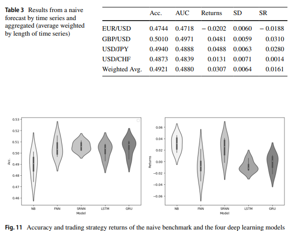
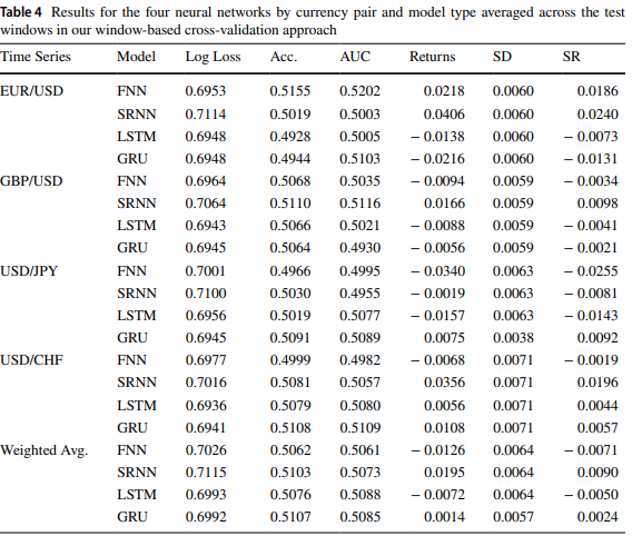
Once we have runed the ONNX_GRU.py, we will get a ONNX model in the same folder we have the traning python file (ONNX_GRU.py). This ONNX model, should be saved in the MQL5 Files folder, to call it from the EA.

This is how the EA is added to the article.

Now we can test the model with the strategy tester or trade.

Comparing GRU vs LSTM

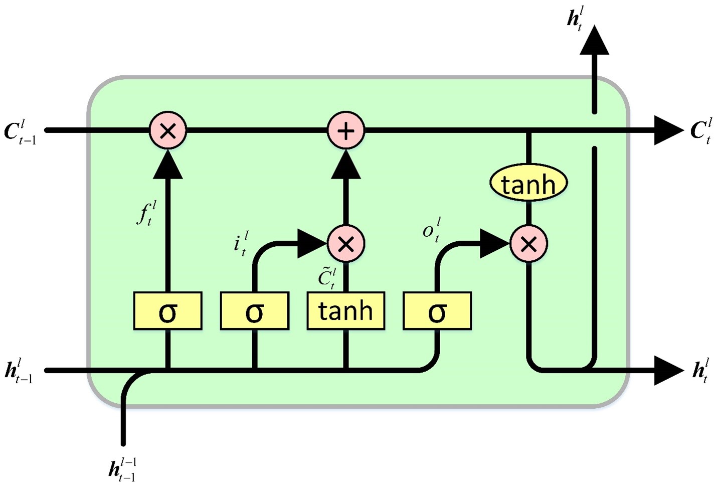
The LSTM cell sustains a cell state, which it both reads from and writes to. It encompasses four gates that govern the processes of reading, writing, and outputting values to and from the cell state, contingent on the input and cell state values. The initial gate dictates the information the hidden state should forget. The subsequent gate is accountable for identifying the segment of the cell state to be written. The third gate determines the contents to be inscribed. Lastly, the last gate retrieves information from the cell state to generate an output.

The GRU cell bears similarities to the LSTM cell, yet it incorporates a few significant distinctions. Firstly, it lacks a hidden state, as the functionality of the hidden state in the LSTM cell design is assumed by the cell state. Subsequently, the processes of deciding what the cell state forgets and which part of the cell state is written to are amalgamated into a singular gate. Only the section of the cell state that has been erased is then inscribed. Lastly, the entire cell state serves as an output, deviating from the LSTM cell, which selectively reads from the cell state to generate an output. These collective modifications result in a more straightforward design with fewer parameters compared to the LSTM. However, the reduction in parameters may potentially lead to a decrease in expressibility.

Experimental Comparison

GRU

# Split the data into training and testing sets
x_train, x_test, y_train, y_test = train_test_split(x_features, y_target, test_size=0.2, shuffle=False)


# Standardize the features StandardScaler()
scaler = StandardScaler()
X_train_scaled = scaler.fit_transform(x_train)
X_test_scaled = scaler.transform(x_test)

scaler_y = StandardScaler()
y_train_scaled = scaler_y.fit_transform(np.array(y_train).reshape(-1, 1))
y_test_scaled = scaler_y.transform(np.array(y_test).reshape(-1, 1))

# Define parameters

learning_rate = 0.001
dropout_rate = 0.5
batch_size = 1024
layer_1 = 256
epochs = 1000
k_reg = 0.001
patience = 10
factor = 0.5
n_splits = 5  # Number of K-fold Splits
window_size = days  # Ajusta esto según tus necesidades

def create_windows(data, window_size):
    return [data[i:i + window_size] for i in range(len(data) - window_size + 1)]

custom_optimizer = Adam(learning_rate=learning_rate)
reduce_lr = ReduceLROnPlateau(monitor='val_loss', factor=factor, patience=patience, min_lr=1e-26)

def build_model(input_shape, k_reg):
    model = Sequential()
    
    layer_sizes = [ 512,1024,512, 256, 128, 64]
    model.add(Dense(layer_1, kernel_regularizer=l2(k_reg), input_shape=input_shape))
    for size in layer_sizes:
        model.add(Dense(size, kernel_regularizer=l2(k_reg)))
        model.add(BatchNormalization())
        model.add(Activation('relu'))
        model.add(Dropout(dropout_rate))

    model.add(Dense(1, activation='linear'))
    model.add(BatchNormalization())
    model.compile(optimizer=custom_optimizer, loss='mse', metrics=[rmse()])
    
    return model



# Define EarlyStopping callback
early_stopping = EarlyStopping(monitor='val_loss', patience=patience, restore_best_weights=True)

# KFold Cross Validation
kfold = KFold(n_splits=n_splits, shuffle=True, random_state=42)
history = []
loss_per_epoch = []
val_loss_per_epoch = []

for train, val in kfold.split(X_train_scaled, y_train_scaled):
    x_train_fold, x_val_fold = X_train_scaled[train], X_train_scaled[val]
    y_train_fold, y_val_fold = y_train_scaled[train], y_train_scaled[val]
    
    # Flatten the input data
    x_train_fold_flat = x_train_fold.flatten()
    x_val_fold_flat = x_val_fold.flatten()

    # Create windows for training and validation
    x_train_windows = create_windows(x_train_fold_flat, window_size)
    x_val_windows = create_windows(x_val_fold_flat, window_size)

    # Rebuild the model
    model = build_model((window_size, 1), k_reg)

    # Create a new optimizer
    custom_optimizer = Adam(learning_rate=learning_rate)
    
    # Recompile the model
    model.compile(optimizer=custom_optimizer, loss='mse', metrics=[rmse()])
    
    hist = model.fit(
        np.array(x_train_windows), y_train_fold[window_size - 1:],
        epochs=epochs,
        validation_data=(np.array(x_val_windows), y_val_fold[window_size - 1:]),
        batch_size=batch_size,
        callbacks=[reduce_lr, early_stopping]
    )
    history.append(hist)
    loss_per_epoch.append(hist.history['loss'])
    val_loss_per_epoch.append(hist.history['val_loss'])




mean_loss_per_epoch = [np.mean(loss) for loss in loss_per_epoch]
val_mean_loss_per_epoch = [np.mean(val_loss) for val_loss in val_loss_per_epoch]

print("mean_loss_per_epoch", mean_loss_per_epoch)
print("unique_min_val_loss_per_epoch", val_loss_per_epoch)

# Create a DataFrame to display the mean loss values
epoch_df = pd.DataFrame({
    'Epoch': range(1, len(mean_loss_per_epoch) + 1),
    'Train Loss': mean_loss_per_epoch,
    'Validation Loss': val_loss_per_epoch
})

LSTM

model = Sequential()
model.add(Conv1D(filters=256, kernel_size=2, activation='relu',padding = 'same',input_shape=(inp_history_size,1)))
model.add(MaxPooling1D(pool_size=2))
model.add(LSTM(100, return_sequences = True))
model.add(Dropout(0.3))
model.add(LSTM(100, return_sequences = False))
model.add(Dropout(0.3))
model.add(Dense(units=1, activation = 'sigmoid'))
model.compile(optimizer='adam', loss= 'mse' , metrics = [rmse()])

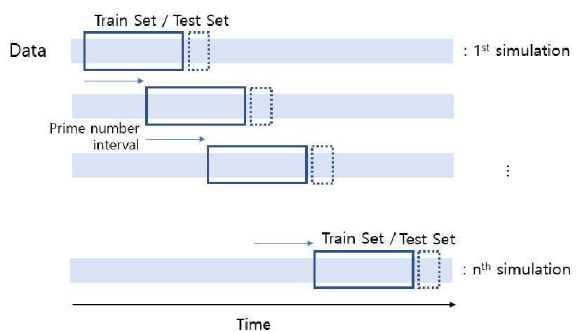
I've left a .py for you to compare LSTM and GRU and a cross validation.py.

Also left a GRU simple .py to make ONNX models

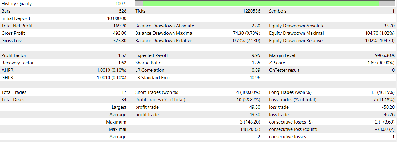
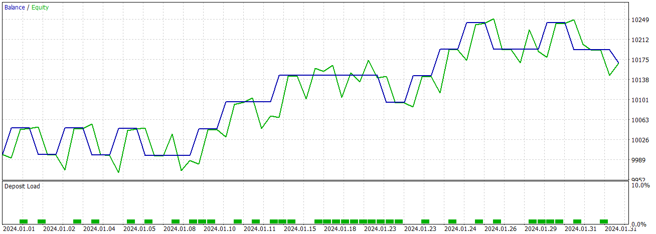
With the simple model that's at the GRU simple, we can get this results over January 2024

Conclusion and Future Work

This comparison is crucial in determining which model to use, or we may even consider using both in a stacked or overlaid fashion. This approach allows us to extract essential information from the models we employ, despite the inherent differences in batch sizes and layer configurations. If as I think they resume in similar results, GRU is much faster.

As part of future work, it would be beneficial to explore different kernel and recurrent initializers tailored to each cell type for potential performance enhancements.

A good approach for trading with ONNX models would be integrating both in the same EA, please read this article: An example of how to ensemble ONNX models in mql5.

Conclusion

Models like GRU are capable of getting good results, and look robust. I hope you have enjoyed this article as much as I have relished creating it. We also have seen the comparison between GRU and LSTM models, and we can use that .py code to know when to stop the epochs (taking into account the number of data for input).

Disclaimer

The past performance does not indicate future results.