
Studying the CCanvas Class. Anti-aliasing and Shadows
Table of Contents
- Introduction
- 1. Coordinates and canvas
- 2. Anti-aliasing algorithm
- 3. Shadow of objects
- 4. Example of the Gaussian blur algorithm
- 5. Class for drawing shadows
- Conclusion
Introduction
I believe that displaying various dynamic effects is one of the issues that can be solved when drawing with the CCanvas class. For example, implementing graphic constructions through the anti-aliasing algorithm gives them a more attractive look. Or drawing a new style of displaying the indicator line called spline. Or maybe drawing a dynamic indicator in a separate window, somehow similar to drawing frequency characteristics on the oscilloscope. In any case, drawing opens up new horizons of application in personal developments.
1. Coordinates and canvas
Canvas is built in the chart's coordinates. In this case a chart size is measured in pixels. The upper left corner of the chart has the coordinates (0,0).
Please note that when drawing on canvas the coordinates of primitives and colored primitives are given exclusively in int. And as for drawing primitives using the anti-aliasing method PixelSetAA, coordinates are given in double, coordinates in the CircleAA method are given in int, and the size of the circle — in double.
| Method | Coordinates | Size |
|---|---|---|
| PixelSetAA | double | - |
| LineAA | int | - |
| PolylineAA | int | - |
| PolygonAA | int | - |
| TriangleAA | int | - |
| CircleAA | int | double |
That is, when giving coordinates for the PixelSetAA method, coordinates of the point can be similar to: (120.3, 25.56). The PixelSetAA.mq5 script draws two columns of eleven points. In the left column the increment for each point along the X axis is 0.1, and the increment along the Y axis is 3.0. In the right column the increment for each point along the X axis is 0.1, and the increment along the Y axis is 3.1.
In order to see how these points are drawn, the operation results of the PixelSetAA.mq5 script were zoomed in multiple times:
![]()
Fig. 1. The PixelSetAA method operation
For a better view I have added borders of anti-aliasing and the text with coordinates for drawing:
![]()
Fig. 2. Visual operation of the PixelSetAA method
As you can see, the pixel is colored with the given color only in the coordinates without fraction. However, if the point has one of the coordinates with fraction, then this point will be drawn with two pixels using different color saturation (left column).
In cases when both coordinates of a point are given with fraction, then such point is drawn with three pixels that have various color saturation (right column). This particular drawing with three pixels but various color saturation allows to achieve the smoothing effect.
2. Anti-aliasing algorithm
Methods of the CCanvas class that draw primitives with anti-aliasing use the common calculation of the point's color method PixelSetAA for displaying on the screen.
| Method | The final method of image calculation |
|---|---|
| PixelSetAA | PixelSetAA |
| LineAA | PixelSetAA |
| PolylineAA | LineAA -> PixelSetAA |
| PolygonAA | LineAA -> PixelSetAA |
| TriangleAA | LineAA -> PixelSetAA |
| CircleAA | PixelSetAA |
The demonstration of a drawing method with anti-aliasing PixelSetAA was seen on the fig. 1.
It turns out that when drawing with anti-aliasing, the PixelSetAA method acts as a base of the CCanvas class. Therefore, I believe it will be interesting to find out how the anti-aliasing algorithm is implemented exactly.
Let me remind you, that the coordinates X and Y of the PixelSetAA method have a double type, thus, the PixelSetAA method can take the coordinates of the point located between pixels:
//+------------------------------------------------------------------+
//| Draw pixel with antialiasing                                     |
//+------------------------------------------------------------------+
void CCanvas::PixelSetAA(const double x,const double y,const uint clr)
  {
Next we are going to declare three arrays. The rr[] array is an auxiliary array for calculating how much a virtual pixel (that can be drawn) covers the physical pixels of the screen. The arrays xx[] and yy[] are the coordinate arrays used for drawing pixels in order to give a smoothing effect to the image.
void CCanvas::PixelSetAA(const double x,const double y,const uint clr)
  {
   static double rr[4];
   static int    xx[4];
   static int    yy[4];
The figure below demonstrates the connection between a virtual pixel and a coverage of physical pixels:
![]()
Fig. 3. Coverage of physical pixels
That means a virtual pixel (with calculated coordinates) frequently has coordinates with a fraction and can cover four physical pixels simultaneously. In this case the anti-aliasing algorithm requires to perform its main duty — color these four physical pixels with a virtual pixel's color, but using different iterations. This way it will deceive our vision — eyes will see a slightly blurred image with a mild color blend and soft borders.
The next block contains preliminary calculations. We obtain values of incoming coordinates rounded to the nearest integer:
static int    yy[4];
//--- preliminary calculations
   int    ix=(int)MathRound(x);
   int    iy=(int)MathRound(y);
For a better understanding how a mathematical function MathRound works (rounding up or down, if the number has a fraction ".5"), it is recommended to run this code:
void OnStart()
  {
   Print("MathRound(3.2)=",DoubleToString(MathRound(3.2),8),"; (int)MathRound(3.2)=",IntegerToString((int)MathRound(3.2)));
   Print("MathRound(3.5)=",DoubleToString(MathRound(3.5),8),"; (int)MathRound(3.5)=",IntegerToString((int)MathRound(3.5)));
   Print("MathRound(3.8)=",DoubleToString(MathRound(3.8),8),"; (int)MathRound(3.8)=",IntegerToString((int)MathRound(3.8)));
  }
//+------------------------------------------------------------------+
and the execution result
MathRound(3.8)=4.00000000; (int)MathRound(3.8)=4
MathRound(3.5)=4.00000000; (int)MathRound(3.5)=4
MathRound(3.2)=3.00000000; (int)MathRound(3.2)=3
Followed by the calculation of dx and dy delta — difference between incoming coordinates x and y and their rounded values ix and iy:
int    iy=(int)MathRound(y);
   double rrr=0;
   double k;
   double dx=x-ix;
   double dy=y-iy;
Now we have to check: if both dx and dy equal to zero, then we exit the PixelSetAA method.
double dy=y-iy;
   uchar  a,r,g,b;
   uint   c;
//--- no need for anti-aliasing
   if(dx==0.0 && dy==0.0)
     {
      PixelSet(ix,iy,clr);
      return;
     }
If deltas are not equal to zero, then we are going to proceed with preparing a pixel array:
PixelSet(ix,iy,clr);
      return;
     }
//--- prepare array of pixels
   xx[0]=xx[2]=ix;
   yy[0]=yy[1]=iy;
   if(dx<0.0)
      xx[1]=xx[3]=ix-1;
   if(dx==0.0)
      xx[1]=xx[3]=ix;
   if(dx>0.0)
      xx[1]=xx[3]=ix+1;
   if(dy<0.0)
      yy[2]=yy[2]=iy-1;
   if(dy==0.0)
      yy[2]=yy[2]=iy;
   if(dy>0.0)
      yy[2]=yy[2]=iy+1;
This block specifically creates a basis for the illusion of a smoothed image.
To visualize operation of this block I wrote a PrepareArrayPixels.mq5 script and recorded a video explaining how it works:
Video 1. Operation of the PrepareArrayPixels.mq5 script
After the pixel array is filled, "weights" are calculated to see how does a virtual pixel cover real pixels:
yy[2]=yy[2]=iy+1;
//--- calculate radii and sum of their squares
   for(int i=0;i<4;i++)
     {
      dx=xx[i]-x;
      dy=yy[i]-y;
      rr[i]=1/(dx*dx+dy*dy);
      rrr+=rr[i];
     }
And the final step — drawing a blur:
rrr+=rr[i];
     }
//--- draw pixels
   for(int i=0;i<4;i++)
     {
      k=rr[i]/rrr;
      c=PixelGet(xx[i],yy[i]);
      a=(uchar)(k*GETRGBA(clr)+(1-k)*GETRGBA(c));
      r=(uchar)(k*GETRGBR(clr)+(1-k)*GETRGBR(c));
      g=(uchar)(k*GETRGBG(clr)+(1-k)*GETRGBG(c));
      b=(uchar)(k*GETRGBB(clr)+(1-k)*GETRGBB(c));
      PixelSet(xx[i],yy[i],ARGB(a,r,g,b));
     }
3. Shadow of objects
Drawing shadows gives softer contour outline to graphic objects, thus creating a minor volume effect, so graphic objects stop looking flat. Furthermore, shadows have a very interesting and beneficial property: shadows of the objects normally are transparent, and upon superposition of graphics with shadows additional volume is created.
The most common types of shadows are shown below:
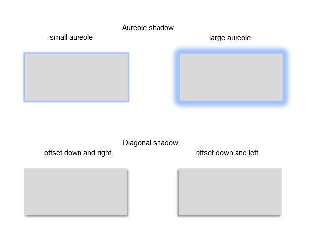
Fig. 4. Types of shadows
An "aureole" shadow may have a setting for an aureole width. An "external diagonal" shadow may have a setting for an angle where a shadow is shifted to. Both types of shadows have color selecting settings.
To select a relevant algorithm for drawing shadows, we must see what does a shade consist of. This is where it comes handy zooming in the image. See below how shadows from the image 4 look at much closer examination:
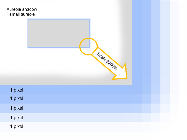
Fig. 5. What a shadow consists of
It becomes clear now that the "aureole" shadow is built from several outlines 1 pixel wide. These outlines have a gradual change of the color saturation.
3.2. Getting normal distribution
To get a smooth transition when drawing a shadow, we are going to use the most common graphic filter — the Gaussian blur (information about the Gaussian blur algorithm is provided below). This filter uses normal distribution when calculating transformations applied to every pixel of the image. The blur calculation of each pixel of the image depends on the blurring radius (the parameter is given before using filter) and must be performed with due attention to all surrounding pixels.
Despite the fact that a blurring radius was mentioned, in fact a pixel grid N x N is used for calculation:
![]()
where Radius is a blurring radius.
The figure below shows an example of a pixel grid for a blurring radius equal to 3.
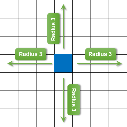
Fig. 6. Blurring radius
I am not going to cover the fast calculation theory for this filter, and will only mention that a separability property of the Gaussian filter will be used: first we apply blurring along the X axis, and then proceed to the Y axis. It helps making calculation faster, without affecting quality.
The influence of adjacent pixels to the calculated pixel is uneven and uses normal distribution for calculation. The further from the calculated pixel a pixel is, the less significant is the effect on it. To calculate normal distribution through the Gaussian algorithm we will use the numerical analysis library ALGLIB. A GQGenerateRecToExel.mq5 script will help us clearly demonstrate a normal distribution modeling. Using the ALGLIB library this script receives an array of weighing coefficients of normal distribution and displays these values in the file <data catalogue>\MQL5\Files\GQGenerateRecToExel.csv. And this is a how the chart built on the basis of the GQGenerateRecToExel.csv file data looks:
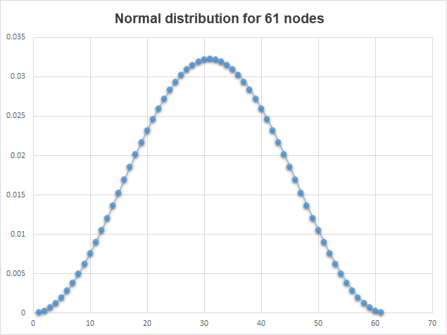
Fig. 7. Normal distribution
Using the GQGenerateRecToExel.mq5 script as an example, we will check the example of obtaining the array of weighting coefficients of a normal distribution. The same GetQuadratureWeights function will be used in the scripts from this point onward:
//+------------------------------------------------------------------+
//| Gets array of quadrature weights                                 |
//+------------------------------------------------------------------+
bool GetQuadratureWeights(const double mu0,const int n,double &w[])
  {
   CAlglib alglib;            // static member of class CAlglib
   double      alp[];         // array alpha coefficients
   double      bet[];         // array beta coefficients
   ArrayResize(alp,n);
   ArrayResize(bet,n);
   ArrayInitialize(alp,1.0);  // initializes a numeric array alpha
   ArrayInitialize(bet,1.0);  // initializes a numeric array beta

   double      out_x[];
   int         inf=0;
//| Info    -   error code:                                          |
//|                 * -3    internal eigenproblem solver hasn't      |
//|                         converged                                |
//|                 * -2    Beta[i]<=0                               |
//|                 * -1    incorrect N was passed                   |
//|                 *  1    OK                                       |
   alglib.GQGenerateRec(alp,bet,mu0,n,inf,out_x,w);
   if(inf!=1)
     {
      Print("Call error in CGaussQ::GQGenerateRec");
      return(false);
     }
   return(true);
  }
This function fills the w[] array with weighing coefficients of normal distribution and also checks the result of calling the ALGLIB library function through the analysis of the inf variable.
When drawing a shadow on canvas, operations with resources (ResourceReadImage) are being used, for example, reading data from the graphical resource and filling the array with this data.
While working with resources you should pay attention that pixel arrays are saved in the uint format (read more: ARGB color representation). You should also know how 2D images with width and height are converted to a one-dimensional array. An algorithm for conversion is the following: subsequent gluing of rows of the image in one long row. The figure below shows two images with size 4 x 3 pixels and 3 x 4 pixels that are converted to a one-dimensional array:
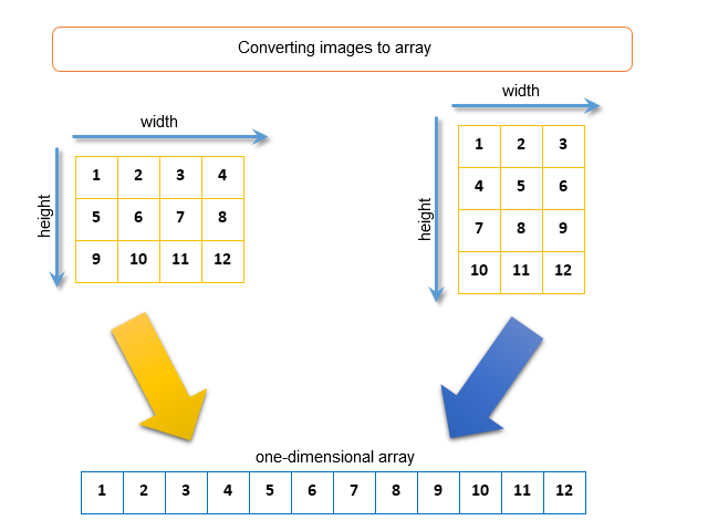
Fig. 8. Converting the image to a one-dimensional array
4. Example of the Gaussian blur algorithm
A Gaussian blur will be considered by applying the ShadowTwoLayers.mq5 algorithm. Two include files Canvas.mqh and the numerical analysis library ALGLIB are required for script operation:
#property script_show_inputs
#include <Canvas\Canvas.mqh>
#include <Math\Alglib\alglib.mqh>
Input parameters:
//--- input
input uint  radius=4;               // radius blur
input color clrShadow=clrBlack;     // shadow color
input uchar ShadowTransparence=160; // transparency shadows
input int   ShadowShift=3;          // shadow shift
input color clrDraw=clrBlue;        // shadow color
input uchar DrawwTransparence=255;  // transparency draws
//---
We will create two canvases. The lower canvas will perform the function of a layer used to draw a shadow, and the upper canvas will act as a working layer for drawing graphic figures. The sizes of both canvases are equal to the size of the chart (a description of the function for obtaining the chart's height and width in pixels is not given here, since these examples are available in the documentation section Examples of working with the chart):
//--- create canvas
   CCanvas CanvasShadow;
   CCanvas CanvasDraw;
   if(!CanvasShadow.CreateBitmapLabel("ShadowLayer",0,0,ChartWidth,
      ChartHeight,COLOR_FORMAT_ARGB_NORMALIZE))
     {
      Print("Error creating canvas: ",GetLastError());
      return;
     }
   if(!CanvasDraw.CreateBitmapLabel("DrawLayer",0,0,ChartWidth
      ,ChartHeight,COLOR_FORMAT_ARGB_NORMALIZE))
     {
      Print("Error creating canvas: ",GetLastError());
      return;
     }
Now let's draw on canvas a little bit. First we will draw a work piece of the shadow figures (shadows are drawn transparent by default) on the lower canvas, and then draw a rectangle on the upper canvas.
//--- draw on canvas
   CanvasShadow.Erase(ColorToARGB(clrNONE,0));
   CanvasShadow.FillRectangle(ChartWidth/10,ChartHeight/10,
                              ChartWidth/2-ChartWidth/10,ChartHeight/10*9,ColorToARGB(clrShadow,ShadowTransparence));
   CanvasShadow.FillRectangle(ChartWidth/2,ChartHeight/12,ChartWidth/3*2,
                              ChartHeight/2,ColorToARGB(clrShadow,ShadowTransparence));
   CanvasShadow.Update();

   CanvasDraw.Erase(ColorToARGB(clrNONE,0));
   CanvasDraw.FillRectangle(ChartWidth/10-ShadowShift,ChartHeight/10-ShadowShift,ChartWidth/2-ChartWidth/10-ShadowShift,
                            ChartHeight/10*9-ShadowShift,ColorToARGB(clrDraw,DrawwTransparence));
   CanvasDraw.Update();
We should get the following image (attention: rectangular "shadows" are not blurred yet):
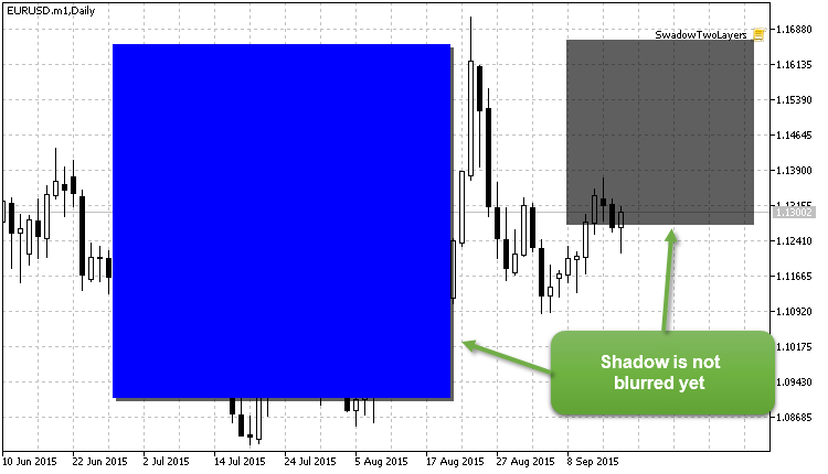
Fig. 9. Shadows are not blurred yet
Blurring will be performed on the lower canvas (CanvasShadow). For this purpose you must read data (ResourceReadImage) from the graphic resource of the lower canvas (CanvasShadow.ResourceName()) and fill in a one-dimensional array (res_data) with this data:
//+------------------------------------------------------------------+
//| reads data from the graphical resource                           |
//+------------------------------------------------------------------+
   ResetLastError();
   if(!ResourceReadImage(CanvasShadow.ResourceName(),res_data,res_width,res_height))
     {
      Print("Error reading data from the graphical resource ",GetLastError());
      Print("attempt number two");
      //--- attempt number two: now the picture width and height are known
      ResetLastError();
      if(!ResourceReadImage(CanvasShadow.ResourceName(),res_data,res_width,res_height))
        {
         Print("Error reading data from the graphical resource ",GetLastError());
         return;
        }
     }
The next step involves getting the array of weighing coefficients of normal distribution through the GetQuadratureWeights function and decomposing the one-dimensional array into four arrays: Alfa, Red, Green and Blue. Color decomposition is mainly required because graphic effects must be applied for each color component.
//+------------------------------------------------------------------+
//| decomposition of pictures on the components r, g, b              |
//+------------------------------------------------------------------+
...
   if(!GetQuadratureWeights(1,NNodes,weights))
      return;

   for(int i=0;i<size;i++)
     {
      clr_temp=res_data[i];
      a_data[i]=GETRGBA(clr_temp);
      r_data[i]=GETRGBR(clr_temp);
      g_data[i]=GETRGBG(clr_temp);
      b_data[i]=GETRGBB(clr_temp);
     }
The following code section is responsible for a blurring "magic". At first, the image will be blurred along the X axis, followed by the same process along the Y axis. This approach follows from the separability property of the Gaussian filter, which allows speeding up calculations without compromising quality. Let's see the example of blurring along the X axis of the image:
//+------------------------------------------------------------------+
//| blur horizontal (axis X)                                         |
//+------------------------------------------------------------------+
   uint XY;             // pixel coordinate in the array
   double   a_temp=0.0,r_temp=0.0,g_temp=0.0,b_temp=0.0;
   int      coef=0;
   int      j=(int)radius;
   for(uint Y=0;Y<res_height;Y++)                  // cycle on image width
     {
      for(uint X=radius;X<res_width-radius;X++)    // cycle on image height
        {
         XY=Y*res_width+X;
         a_temp=0.0; r_temp=0.0; g_temp=0.0; b_temp=0.0;
         coef=0;
         for(int i=-1*j;i<j+1;i=i+1)
           {
            a_temp+=a_data[XY+i]*weights[coef];
            r_temp+=r_data[XY+i]*weights[coef];
            g_temp+=g_data[XY+i]*weights[coef];
            b_temp+=b_data[XY+i]*weights[coef];
            coef++;
           }
         a_data[XY]=(uchar)MathRound(a_temp);
         r_data[XY]=(uchar)MathRound(r_temp);
         g_data[XY]=(uchar)MathRound(g_temp);
         b_data[XY]=(uchar)MathRound(b_temp);
        }
      //--- remove artifacts on the left
      for(uint x=0;x<radius;x++)
        {
         XY=Y*res_width+x;
         a_data[XY]=a_data[Y*res_width+radius];
         r_data[XY]=r_data[Y*res_width+radius];
         g_data[XY]=g_data[Y*res_width+radius];
         b_data[XY]=b_data[Y*res_width+radius];
        }
      //--- remove artifacts on the right
      for(uint x=res_width-radius;x<res_width;x++)
        {
         XY=Y*res_width+x;
         a_data[XY]=a_data[(Y+1)*res_width-radius-1];
         r_data[XY]=r_data[(Y+1)*res_width-radius-1];
         g_data[XY]=g_data[(Y+1)*res_width-radius-1];
         b_data[XY]=b_data[(Y+1)*res_width-radius-1];
        }
     }
So we see two nested loops:
for(uint Y=0;Y<res_height;Y++)                  // cycle on image width
     {
      for(uint X=radius;X<res_width-radius;X++)    // cycle on image height
        {
         ...
        }
     }
This nesting ensures a passage through each pixel of the image:
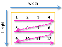
Fig. 10. Pass through each pixel of the image
A nested loop ensures the calculation of blurring along the X axis for each pixel:
for(uint X=radius;X<res_width-radius;X++)    // cycle on image height
        {
         XY=Y*res_width+X;
         a_temp=0.0; r_temp=0.0; g_temp=0.0; b_temp=0.0;
         coef=0;
         for(int i=-1*j;i<j+1;i=i+1)
           {
            a_temp+=a_data[XY+i]*weights[coef];
            r_temp+=r_data[XY+i]*weights[coef];
            g_temp+=g_data[XY+i]*weights[coef];
            b_temp+=b_data[XY+i]*weights[coef];
            coef++;
           }
         a_data[XY]=(uchar)MathRound(a_temp);
         r_data[XY]=(uchar)MathRound(r_temp);
         g_data[XY]=(uchar)MathRound(g_temp);
         b_data[XY]=(uchar)MathRound(b_temp);
        }
The amount of adjunct pixels equal to the blurring radius is selected for every pixel on the left and on the right. Let me remind you, that previously we used the GetQuadratureWeights function to obtain the array of weighting coefficients of normal distribution. The following compatibility is obtained: number of adjacent pixels on the left + pixel for which calculation of blurring is performed + number of adjacent pixels on the right = number of the array elements of weighting coefficients. This way, each adjacent pixel corresponds to a specific value in the array of weighting coefficients.
This is how blurring is calculated for each color: every adjacent pixel is multiplied by the weighting coefficient corresponding to it, and the obtained values are summarized. There is an example below to calculate the image blurring in red where blurring radius equals 4:
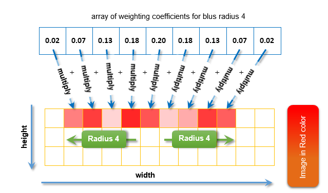
Fig. 11. Calculation of blurring
Artifacts, that are stripes of pixels that were not blurred, remain along the edges of the image when applying the blurring algorithm. A width of these stripes equals the blurring radius. The larger the blurring radius is, the wider the stripes of pixels that were not blurred are. In the algorithm these artifacts are removed by copying the blurred pixels:
//--- remove artifacts on the left
      for(uint x=0;x<radius;x++)
        {
         XY=Y*res_width+x;
         a_data[XY]=a_data[Y*res_width+radius];
         r_data[XY]=r_data[Y*res_width+radius];
         g_data[XY]=g_data[Y*res_width+radius];
         b_data[XY]=b_data[Y*res_width+radius];
        }
      //--- remove artifacts on the right
      for(uint x=res_width-radius;x<res_width;x++)
        {
         XY=Y*res_width+x;
         a_data[XY]=a_data[(Y+1)*res_width-radius-1];
         r_data[XY]=r_data[(Y+1)*res_width-radius-1];
         g_data[XY]=g_data[(Y+1)*res_width-radius-1];
         b_data[XY]=b_data[(Y+1)*res_width-radius-1];
        }
Similar blurring operations are performed for the Y axis. As a result, we get four arrays a1_data[], r1_data[], g1_data[], b1_data[] that have blurred values written for Alpha, red, green and blue, respectively. It remains to collect color from these four components for each pixel and apply it to CanvasShadow canvas:
//---
   for(int i=0;i<size;i++)
     {
      clr_temp=ARGB(a1_data[i],r1_data[i],g1_data[i],b1_data[i]);
      res_data[i]=clr_temp;
     }
   for(uint X=0;X<res_width;X++)
     {
      for(uint Y=radius;Y<res_height-radius;Y++)
        {
         XY=Y*res_width+X;
         CanvasShadow.PixelSet(X,Y,res_data[XY]);
        }
     }
   CanvasShadow.Update();
   CanvasDraw.Update();
   Sleep(21000);
The result of blurring a layer with shadows:
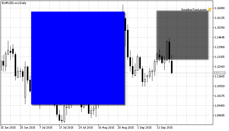
Fig. 12. Shadows are now blurred
5. Class for drawing shadows
The example of drawing on canvas is implemented in the CGauss class. The CGauss class allows drawing such primitives with shadows:
| Primitives | Description |
|---|---|
| LineVertical | Draws vertical line with a shadow |
| LineHorizontal | Draws horizontal line with a shadow |
| Line | Draws arbitrary line with a shadow |
| Polyline | Draws polyline with a shadow |
| Polygon | Draws polygon with a shadow |
| Rectangle | Draws rectangle with a shadow |
| Circle | Draws circle with a shadow |
| FillRectangle | Draws filled rectangle with a shadow |
| FillTriangle | Draws filled triangle with a shadow |
| FillPolygon | Draws filled polygon with a shadow |
| FillCircle | Draws filled circle with a shadow |
| FillEllipse | Draws filled ellipse with a shadow |
| Fill | Fills area with a shadow |
| TextOut | Displays text with a shadow |
Demonstration video of the Blur.mq5 script that draws primitives with shadows:
Video 2. Drawing primitives with shadows
The numerical analysis library ALGLIB is used for calculating shadow color in the CGauss class. There is one shadow type implemented in this class — a shadow drawn outside diagonally below on the right with a shift (see fig. 4).
The general idea of the CGauss is to create two canvases. The lower canvas will perform the function of a layer used to draw a shadow, and the upper canvas will act as a working layer for drawing graphic figures. Sizes of both canvases equal the size of the chart. Wherein lower canvas, when created, is shifted horizontally and vertically by the size of a shadow displacement — this way the calculation of coordinates for drawing shadows becomes easier.
The shadow drawing algorithm operates by the following principle: the amount of objects equal to the blurring radius is subsequently drawn on the lower canvas. The color of each object is calculated through the Gaussian algorithm, thus obtaining a subtle graduation from the given shadow color to complete transparency.
Conclusion
In this article, we have covered the anti-aliasing algorithm in the CCanvas class, along with the examples of calculations and drawing blurring and shadows of the objects. Herewith, the numerical analysis library ALGLIB was applied in calculations of forming blurs and shades.
In addition to that, the CGauss class for drawing graphic primitives with shadows was written based on various examples.
Translated from Russian by MetaQuotes Ltd.
Original article: https://www.mql5.com/ru/articles/1612
 Graphical Interfaces I: Functions for the Form Buttons and Deleting Interface Elements (Chapter 4)
 Graphical Interfaces I: Animating the Graphical Interface (Chapter 3)
 Trading signals module using the system by Bill Williams
- Free trading apps
- Over 8,000 signals for copying
- Economic news for exploring financial markets
You agree to website policy and terms of use