
Neural networks made easy (Part 4): Recurrent networks
Contents
- Introduction
- 1. Distinctive features of recurrent neural networks
- 2. Recurrent network training principles
- 3. Building a recurrent neural network
- 3.1. Class initialization method
- 3.2. Feed-forward
- 3.3. Error gradient calculation
- 3.4. Updating the weights
- 4. Testing
- Conclusion
- Links
- Programs used in the article
Introduction
We continue to study neural networks. We have previously discussed the multilayer perceptron and convolutional neural networks. All of them work with static data within the framework of Markov processes, according to which the subsequent system state depends only on its current state and does not depend on the state of the system in the past. Now, I suggest considering Recurrent Neural Networks. This is a special type of neural networks designed to work with time sequences and is considered the leader in this sphere.
1. Distinctive features of recurrent neural networks
All previously discussed types of neural networks work with a predetermined amount of data. However, in our case it is hard to determine the ideal amount of analyzed data for price charts. Different patterns can appear at different time intervals. Even the intervals themselves are not always static and can vary depending on the current situation. Some events may be rare in the market, but they work out with a high degree of probability. It is good when the event is within the analyzed data window. If it falls beyond the analyzed series, the neural network will ignore it, even if the market will be working out a reaction to this event at that very moment. An increase in the analyzed window will lead to an increase in the consumption of computing resources and will require more time to make a decision.
Recurrent neurons in neural networks have been proposed for solving this problem when working with time series. This is an attempt to implement short-term memory in neural networks, when system's current state is fed into a neuron along with the previous state of the same neuron. This procedure is based on the assumption that the value at the neuron output takes into account the influence of all factors (including its previous state) and at the next step it will transfer "all its knowledge" to its future state. This is similar to us, when we act based on our previous experience and earlier performed actions. The memory duration and its influence on the current neuron state will depend on weights.
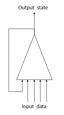
Unfortunately, such a simple solution has its drawbacks. This approach allows saving "memory" for a short time interval. The cyclic multiplication of the signal by a factor less than 1 and the application of the neuron activation function lead to a gradual attenuation of the signal, as the number of cycles increases. To solve this problem, Sepp Hochreiter and Jürgen Schmidhuber proposed in 1997 the use of the Long Short-Term Memory (LSTM) architecture. The LTSM algorithm is considered one of the best solution for the time series classification and forecasting problems, in which significant events are separated in time and stretched over time intervals.
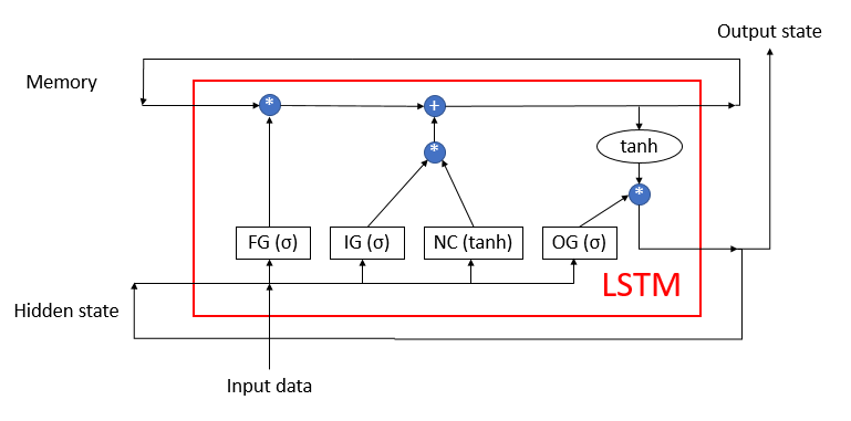
LSTM can hardly be called a neuron. It is already a neural network with 3 input channels and 3 output channels. Data is exchanged with the outside world using only two channels (one for input and the other one for output). The remaining four channels are closed in pairs for cyclic information exchange (Memory and Hidden state).
The LSTM block contains two main data streams which are interconnected by 4 fully connected neural layers. All neural layers contain the same number of neurons, which is equal to the size of the output stream and the memory stream. Let us consider the algorithm in more detail.
The Memory data stream is used to store and transmit important information over time. It is first initialized with zero values and is then filled in during the operation of the neural network. This can be compared to a human being who is born without knowledge and learns throughout his or her life.
The Hidden state stream is intended for transmitting the output system state over time. The data channel size is equal to the "memory" data channel.
Input data and Output stata channels are intended for exchanging information with the outside world.
Three data streams are fed into the algorithm:
- Input data describes the current state of the system.
- Memory and Hidden state are received from the previous state.
At the beginning of the algorithm, information from Input data and Hidden state is combined into a single data array, which is then fed to all 4 hidden neural layers of the LSTM.
The first neural layer, "Forget gate", determines which of the received data in the memory can be forgotten and which should be remembered. It is implemented as a fully connected neural layer with a sigmoid activation function. The number of neurons in the layer corresponds to the number of memory cells in the Memory stream. Each neuron of the layer receives at the input the total array of Input data and Hidden state streams, and it outputs a number in the range from 0 (completely forget) to 1 (save in memory). The element-wise product of the neural layer output data the with the memory stream returns the corrected memory.
At the next step, the algorithm determines which of the data obtained at this step should be stored in memory. The following two neural layers are used for this purpose:
- New Content — a fully connected neural layer with a hyperbolic tangent as an activation function. It normalizes the received information in the range from -1 to 1.
- Input gate - a fully connected neural layer with a sigmoid as an activation function. It is similar to Forget gate and determines which new data to remember.
The element-wise product of New Content and Input gate is added to the memory cell values. As a result of these operations, we obtain an updated memory state, which is then input to the next iteration cycle.
After updating the memory, the values of the output stream should be generated. Here, similarly to Forget gate and Input gate, calculate Output gate, normalize the current memory value using the hyperbolic tangent. The element-wise product of the two received datasets produces the output signal array, which is output from the LSTM to the outside world. The same data array is passed to the next iteration cycle as a hidden state stream.
2. Recurrent network training principles
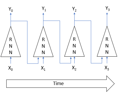
Recurrent neural networks are trained by the already well-known back propagation method. Similarly to the training of convolutional neural networks, the cyclical nature of the process in time is decomposed into a multilayer perceptron. Each time interval in such a perceptron acts as a hidden layer. However, one martix of weights is used for all layers of such a perceptron. Therefore, to adjust the weights, take the sum of gradients for all layers, and calculate the delta of weights once for the total gradient over all layers.
3. Building a recurrent neural network
We will use the LSTM block to build our recurrent neural network. Let us start with the creation of the CNeuronLSTM class. To preserve the class inheritance structure created in the previous article, we will create the new class as an inheritor of the CNeuronProof class.
class CNeuronLSTM    :  public CNeuronProof
  {
protected:
   CLayer            *ForgetGate;
   CLayer            *InputGate;
   CLayer            *OutputGate;
   CLayer            *NewContent;
   CArrayDouble      *Memory;
   CArrayDouble      *Input;
   CArrayDouble      *InputGradient;
   //---
   virtual bool      feedForward(CLayer *prevLayer);
   virtual bool      calcHiddenGradients(CLayer *&nextLayer);
   virtual bool      updateInputWeights(CLayer *&prevLayer);
   virtual bool      updateInputWeights(CLayer *gate, CArrayDouble *input_data);
   virtual bool      InitLayer(CLayer *layer, int numOutputs, int numOutputs);
   virtual CArrayDouble *CalculateGate(CLayer *gate, CArrayDouble *sequence);

public:
                     CNeuronLSTM(void);
                    ~CNeuronLSTM(void);
   virtual bool      Init(uint numOutputs,uint myIndex,int window, int step, int units_count);
   //---
   virtual CLayer    *getOutputLayer(void)  { return OutputLayer;  }
   virtual bool      calcInputGradients(CLayer *prevLayer) ;
   virtual bool      calcInputGradients(CNeuronBase *prevNeuron, uint index) ;
   //--- methods for working with files
   virtual bool      Save( int const file_handle);
   virtual bool      Load( int const file_handle);
   virtual int       Type(void)   const   {  return defNeuronLSTM;   }
  };
The parent class contains a layer of output neurons OutputLayer. Let us add 4 neural layers required for algorithm operation: ForgetGate, InputGate, OutputGate and NewContent. Also add 3 arrays to store "memory" data, to combine Input data and Hidden state, as well as the error gradient of input data. The name and functionality of the class methods correspond to those considered earlier. However, their codes have some differences required for algorithm operation. Let us consider the main methods in more detail.
3.1. Class initialization method.
The class initialization method receives in the parameters the basic information about the block being created. Method parameter names have been inherited from the base class, but some of them now have a different meaning:
- numOutputs — the number of outgoing connections. They are used when a fully connected layer follows the LSTM block layer.
- myIndex — index of a neuron in the layer. It is used for block identification.
- window — Input data channel size.
- step — not used.
- units_count — the width of the output channel and the number of neurons in the hidden layers of the block. All neural layers of a block contain the same number of neurons.
bool CNeuronLSTM::Init(uint numOutputs,uint myIndex,int window,int step,int units_count)
  {
   if(units_count<=0)
      return false;
//--- Init Layers
   if(!CNeuronProof::Init(numOutputs,myIndex,window,step,units_count))
      return false;
   if(!InitLayer(ForgetGate,units_count,window+units_count))
      return false;
   if(!InitLayer(InputGate,units_count,window+units_count))
      return false;
   if(!InitLayer(OutputGate,units_count,window+units_count))
      return false;
   if(!InitLayer(NewContent,units_count,window+units_count))
      return false;
   if(!Memory.Reserve(units_count))
      return false;
   for(int i=0; i<units_count; i++)
      if(!Memory.Add(0))
         return false;
//---
   return true;
  }
Inside the method, we first check that at least one neuron has been created in each neural layer of the block. Then we call the corresponding method of the base class. After the successful completion of the method, initialize the hidden layers of the block, while the operations which repeat for each layer will be provided in a separate method InitLayer. Once the initialization of the neural layers is complete, the memory array is initialized with zero values.
The InitLayer neural layer initialization method receives in parameters a pointer to the object of the initialized neural layer, the number of neurons in the layer and the number of outgoing connections. At the beginning of the method, check the validity of the received pointer. If the pointer is invalid, create a new instance of the neural layer class. If the pointer is valid, clear the layer of neurons.
bool CNeuronLSTM::InitLayer(CLayer *layer,int numUnits, int numOutputs)
  {
   if(CheckPointer(layer)==POINTER_INVALID)
     {
      layer=new CLayer(numOutputs);
      if(CheckPointer(layer)==POINTER_INVALID)
         return false;
     }
   else
      layer.Clear();
Fill the layer with the required number of neurons. If an error occurs at any of the method stages, exit the function with the false result.
   if(!layer.Reserve(numUnits))
      return false;
//---
   CNeuron *temp;
   for(int i=0; i<numUnits; i++)
     {
      temp=new CNeuron();
      if(CheckPointer(temp)==POINTER_INVALID)
         return false;
      if(!temp.Init(numOutputs+1,i))
         return false;
      if(!layer.Add(temp))
         return false;
     }
//---
   return true;
  }
After successful completion of all iterations, exit the method with the true result.
3.2. Feed-forward.
The feed forward pass is implemented in the feedForward method. The method receives in parameters a pointer to the previous neural layer. At the method beginning, check the validity of the received pointer and the availability of neurons in the previous layer. Also check the validity of the array used for the input data. If the object has not been created, create a new instance of the class. If an object already exists, clear the array.
bool CNeuronLSTM::feedForward(CLayer *prevLayer)
  {
   if(CheckPointer(prevLayer)==POINTER_INVALID || prevLayer.Total()<=0)
      return false;
   CNeuronBase *temp;
   CConnection *temp_con;
   if(CheckPointer(Input)==POINTER_INVALID)
     {
      Input=new CArrayDouble();
      if(CheckPointer(Input)==POINTER_INVALID)
         return false;
     }
   else
      Input.Clear();
Next, combine data about the current system state and data about the state at the previous time interval into a single input data array Input.
   int total=prevLayer.Total();
   if(!Input.Reserve(total+OutputLayer.Total()))
      return false;
   for(int i=0; i<total; i++)
     {
      temp=prevLayer.At(i);
      if(CheckPointer(temp)==POINTER_INVALID || !Input.Add(temp.getOutputVal()))
         return false;
     }
   total=OutputLayer.Total();
   for(int i=0; i<total; i++)
     {
      temp=OutputLayer.At(i);
      if(CheckPointer(temp)==POINTER_INVALID || !Input.Add(temp.getOutputVal()))
         return false;
     }
   int total_data=Input.Total();
Calculate the value of the gates. Similarly to initialization, move the operations repeated for each gate into a separate CalculateGate method. Call here this method, inputting into it pointers to the processed gate and the initial data array.
//--- Calculated forget gate
   CArrayDouble *forget_gate=CalculateGate(ForgetGate,Input);
   if(CheckPointer(forget_gate)==POINTER_INVALID)
      return false;
//--- Calculated input gate
   CArrayDouble *input_gate=CalculateGate(InputGate,Input);
   if(CheckPointer(input_gate)==POINTER_INVALID)
      return false;
//--- Calculated output gate
   CArrayDouble *output_gate=CalculateGate(OutputGate,Input);
   if(CheckPointer(output_gate)==POINTER_INVALID)
      return false;
Calculate and normalize incoming data into the new_content array.
//--- Calculated new content
   CArrayDouble *new_content=new CArrayDouble();
   if(CheckPointer(new_content)==POINTER_INVALID)
      return false;
   total=NewContent.Total();
   for(int i=0; i<total; i++)
     {
      temp=NewContent.At(i);
      if(CheckPointer(temp)==POINTER_INVALID)
         return false;
      double val=0;
      for(int c=0; c<total_data; c++)
        {
         temp_con=temp.Connections.At(c);
         if(CheckPointer(temp_con)==POINTER_INVALID)
            return false;
         val+=temp_con.weight*Input.At(c);
        }
      val=TanhFunction(val);
      temp.setOutputVal(val);
      if(!new_content.Add(val))
         return false;
     }
Finally, after all the intermediate calculations, calculate the "memory" array and determine the output data.
//--- Calculated output sequences
   for(int i=0; i<total; i++)
     {
      double value=Memory.At(i)*forget_gate.At(i)+new_content.At(i)*input_gate.At(i);
      if(!Memory.Update(i,value))
         return false;
      temp=OutputLayer.At(i);
      value=TanhFunction(value)*output_gate.At(i);
      temp.setOutputVal(value);
     }
Then, delete intermediate data arrays and exit the method with true.
   delete forget_gate;
   delete input_gate;
   delete new_content;
   delete output_gate;
//---
   return true;
  }
In the above CalculateGate method, the matrix of weights is multiplied by the initial data vector, followed by data normalization through the sigmoid activation function. This method receives in parameters 2 pointers to objects of the neural layer and the original data sequence. First, check the validity of the received pointers.
CArrayDouble *CNeuronLSTM::CalculateGate(CLayer *gate,CArrayDouble *sequence)
  {
   CNeuronBase *temp;
   CConnection *temp_con;
   CArrayDouble *result=new CArrayDouble();
   if(CheckPointer(gate)==POINTER_INVALID)
      return NULL;
Next, implement a loop through all neurons.
   int total=gate.Total();
   int total_data=sequence.Total();
   for(int i=0; i<total; i++)
     {
      temp=gate.At(i);
      if(CheckPointer(temp)==POINTER_INVALID)
        {
         delete result;
         return NULL;
        }
After checking the validity of the pointer to the neuron object, implement a nested loop through all the weights of the neuron, while calculating the sum of the products of the weights by the corresponding element in the initial data array.
      double val=0;
      for(int c=0; c<total_data; c++)
        {
         temp_con=temp.Connections.At(c);
         if(CheckPointer(temp_con)==POINTER_INVALID)
           {
            delete result;
            return NULL;
           }
         val+=temp_con.weight*(sequence.At(c)==DBL_MAX ? 1 : sequence.At(c));
        }
The resulting sum of products is passed through the activation function. The result is written to the neuron output and is added to the array. After successfully iterating over all neurons in the layer, exit the method by returning an array of results. If an error occurred at any calculation stage, the method will return an empty value.
      val=SigmoidFunction(val);
      temp.setOutputVal(val);
      if(!result.Add(val))
        {
         delete result;
         return NULL;
        }
     }
//---
   return result;
  }
3.3. Error gradient calculation.
Error gradients are calculated in the calcHiddenGradients method, which receives a pointer to the next layer of neurons in the parameters. At the method beginning, check the relevance of the previously created object used for storing the sequence of error gradients to the original data. If the object has not yet been created, create a new instance. If an object already exists, clear the array. Also, declare internal variables and class instances.
bool CNeuronLSTM::calcHiddenGradients(CLayer *&nextLayer)
  {
   if(CheckPointer(InputGradient)==POINTER_INVALID)
     {
      InputGradient=new CArrayDouble();
      if(CheckPointer(InputGradient)==POINTER_INVALID)
         return false;
     }
   else
      InputGradient.Clear();
//---
   int total=OutputLayer.Total();
   CNeuron *temp;
   CArrayDouble *MemoryGradient=new CArrayDouble();
   CNeuron *gate;
   CConnection *con;
Next, calculate the error gradient for the output layer of neurons, which came from the next neural layer.
   for(int i=0; i<total; i++)
     {
      temp=OutputLayer.At(i);
      if(CheckPointer(temp)==POINTER_INVALID)
         return false;
      temp.setGradient(temp.sumDOW(nextLayer));
     }
Extend the resulting gradient to all inner neural layers of the LSTM.
   if(CheckPointer(MemoryGradient)==POINTER_INVALID)
      return false;
   if(!MemoryGradient.Reserve(total))
      return false;
   for(int i=0; i<total; i++)
     {
      temp=OutputLayer.At(i);
      gate=OutputGate.At(i);
      if(CheckPointer(gate)==POINTER_INVALID)
         return false;
      double value=temp.getGradient()*gate.getOutputVal();
      value=TanhFunctionDerivative(Memory.At(i))*value;
      if(i>=MemoryGradient.Total())
        {
         if(!MemoryGradient.Add(value))
            return false;
        }
      else
        {
         value=MemoryGradient.At(i)+value;
         if(!MemoryGradient.Update(i,value))
            return false;
        }
      gate.setGradient(gate.getOutputVal()!=0 && temp.getGradient()!=0 ? temp.getGradient()*temp.getOutputVal()*SigmoidFunctionDerivative(gate.getOutputVal())/gate.getOutputVal() : 0);
      //--- Calcculated gates and new content gradients
      gate=ForgetGate.At(i);
      if(CheckPointer(gate)==POINTER_INVALID)
         return false;
      gate.setGradient(gate.getOutputVal()!=0 && value!=0? value*SigmoidFunctionDerivative(gate.getOutputVal()) : 0);
      gate=InputGate.At(i);
      temp=NewContent.At(i);
      if(CheckPointer(gate)==POINTER_INVALID)
         return false;
      gate.setGradient(gate.getOutputVal()!=0 && value!=0 ? value*temp.getOutputVal()*SigmoidFunctionDerivative(gate.getOutputVal()) : 0);
      temp.setGradient(temp.getOutputVal()!=0 && value!=0 ? value*gate.getOutputVal()*TanhFunctionDerivative(temp.getOutputVal()) : 0);
     }
After calculating the gradients on the inner neural layers, calculate the error gradient for the sequence of initial data.
//--- Calculated input gradients
   int total_inp=temp.getConnections().Total();
   for(int n=0; n<total_inp; n++)
     {
      double value=0;
      for(int i=0; i<total; i++)
        {
         temp=ForgetGate.At(i);
         con=temp.getConnections().At(n);
         value+=temp.getGradient()*con.weight;
         //---
         temp=InputGate.At(i);
         con=temp.getConnections().At(n);
         value+=temp.getGradient()*con.weight;
         //---
         temp=OutputGate.At(i);
         con=temp.getConnections().At(n);
         value+=temp.getGradient()*con.weight;
         //---
         temp=NewContent.At(i);
         con=temp.getConnections().At(n);
         value+=temp.getGradient()*con.weight;
        }
      if(InputGradient.Total()>=n)
        {
         if(!InputGradient.Add(value))
            return false;
        }
      else
         if(!InputGradient.Update(n,value))
            return false;
     }
After calculating all gradients, delete unnecessary objects and exit the method with true.
   delete MemoryGradient;
//---
   return true;
  }
Please pay attention the following point: in the theoretical part, I mentioned the need to unroll the sequence in time and to calculate the error gradients at each time stage. This has not been done here, since the used training coefficient is much less than 1, and the influence of the error gradient on the previous time intervals will be so small that it can be ignored to improve the overall performance of the algorithm.
3.4. Updating the weights.
Naturally, after obtaining the error gradients, we need correct the weights of all LSTM neural layers. This task is implemented in the updateInputWeights method, which received a pointer to the previous neural layer in parameters. Please note that inputting of a pointer to the previous layer is only implemented to preserve the inheritance structure.
At the method beginning, check the validity of the received pointer and the availability of the initial data array. After successful validation of pointers, proceed to adjusting the weights of the inner neural layers. Again, the repeating actions are moved into a separate updateInputWeights method, in which parameters we pass pointers to a specific neural layer and an initial data array. Here, the helper method is called successively for each neural layer.
bool CNeuronLSTM::updateInputWeights(CLayer *&prevLayer)
  {
   if(CheckPointer(prevLayer)==POINTER_INVALID || CheckPointer(Input)==POINTER_INVALID)
      return false;
//---
   if(!updateInputWeights(ForgetGate,Input) || !updateInputWeights(InputGate,Input) || !updateInputWeights(OutputGate,Input)
      || !updateInputWeights(NewContent,Input))
     {
      return false;
     }
//---
   return true;
  }
Let us consider the operations performed in the updateInputWeights(CLayer *gate,CArrayDouble *input_data) method. At the method beginning, check the validity of the pointers received in the parameters and declare internal variables.
bool CNeuronLSTM::updateInputWeights(CLayer *gate,CArrayDouble *input_data)
  {
   if(CheckPointer(gate)==POINTER_INVALID || CheckPointer(input_data)==POINTER_INVALID)
      return false;
   CNeuronBase *neuron;
   CConnection *con;
   int total_n=gate.Total();
   int total_data=input_data.Total();
Arrange nested loops to iterate over all neurons in the layer and weights in neurons, with the correction of the weight matrix. The weight adjustment formula is the same that was considered earlier for CNeuron::updateInputWeights(CArrayObj *&prevLayer). However, we cannot use here the previously created method because that time we used neuron connections to connect with the next layer, while now they are used to connect with the previous layer.
   for(int n=0; n<total_n; n++)
     {
      neuron=gate.At(n);
      if(CheckPointer(neuron)==POINTER_INVALID)
         return false;
      for(int i=0; i<total_data; i++)
        {
         con=neuron.getConnections().At(i);
         if(CheckPointer(con)==POINTER_INVALID)
            return false;
         double data=input_data.At(i);
         con.weight+=con.deltaWeight=(neuron.getGradient()!=0 && data!=0 ? eta*neuron.getGradient()*(data!=DBL_MAX ? data : 1) : 0)+alpha*con.deltaWeight;
        }
     }
//---
   return true;
  }
After updating the weight matrix, exit the method with true.
After creating the class, let us make small adjustments to the dispatchers of the CNeuronBase base class so that they can correctly handle the instances of the new class. The full code of all methods and functions is available in the attachment.
4. Testing
The newly created LSTM block was tested under the same conditions that we used for testing convolutional networks in the previous article. The Fractal_LSTM Expert Advisor has been created for testing. Essentially, this is the same Fractal_conv from the previous article. But in the OnInit function, in the network structure specifying block, the convolutional and subsampled layers have been replaced with a layer of 4 LSTM blocks (by analogy with 4 filters of the convolutional network).
      //---
      desc=new CLayerDescription();
      if(CheckPointer(desc)==POINTER_INVALID)
         return INIT_FAILED;
      desc.count=4;
      desc.type=defNeuronLSTM;
      desc.window=(int)HistoryBars*12;
      desc.step=(int)HistoryBars/2;
      if(!Topology.Add(desc))
         return INIT_FAILED;
No other changes have been made to the EA code. Find the entire EA code and classes in the attachment.
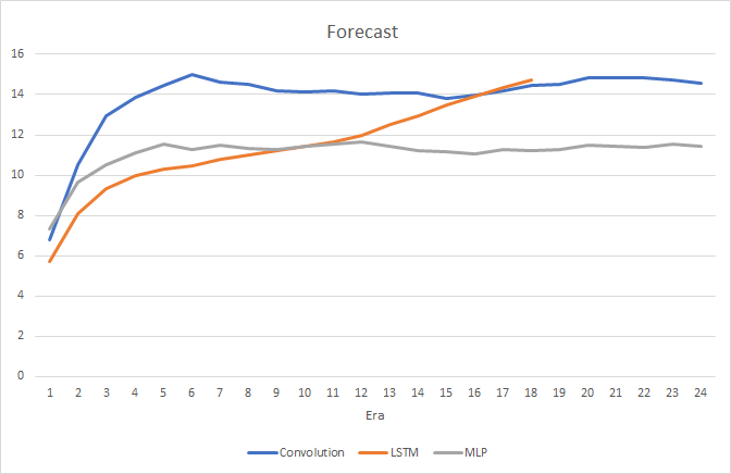
Of course, the use of 4 internal neural layers in each LSTM block and the complexity of the algorithm itself affected the performance, and thus the speed of such a neural network is somewhat lower than the previously considered convolutional network. However, the root mean square error of the recurrent network is much less.
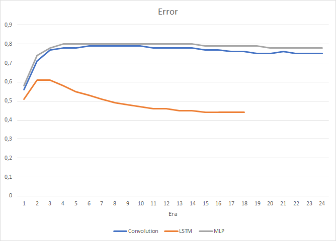
In the process of recurrent neural network training, the target hitting accuracy graph has a pronounced, almost straight, upward trend.
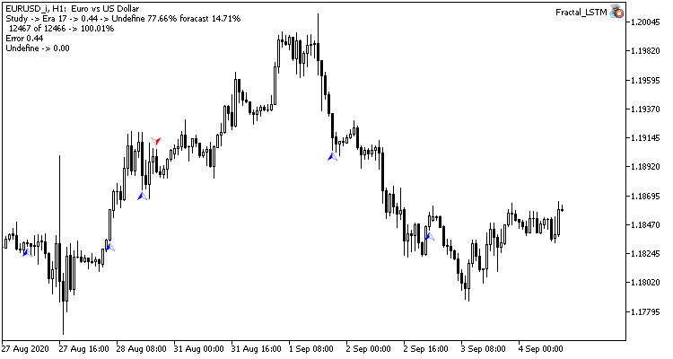
Only rare pointers to predicted fractals are visible on the price chart. In the previous tests, the price chart was full of prediction labels.
Conclusion
In this article, we have examined the algorithm of recurrent neural networks, built an LSTM block and tested the operation of the created neural network using real data. In comparison with the previously considered types of neural networks, recurrent networks are more resource and effort intensive, both during a feed-forward pass and the learning process. Nevertheless, they show better results, which has been confirmed by conducted tests.
Links
- Neural Networks Made Easy
- Neural networks made easy (Part 2): Network training and testing
- Neural networks made easy (Part 3): Convolutional networks
- Understanding LSTM Networks
Programs used in the article
| # | Name | Type | Description |
|---|---|---|---|
| 1 | Fractal.mq5 | Expert Advisor | An Expert Advisor with the regression neural network (1 neuron in the output layer) |
| 2 | Fractal_2.mq5 | Expert Advisor | An Expert Advisor with the classification neural network (3 neurons in the output layer) |
| 3 | NeuroNet.mqh | Class library | A library of classes for creating a neural network (a perceptron) |
| 4 | ractal_conv.mq5 | Expert Advisor | An Expert Advisor with the convolutional neural network (3 neurons in the output layer) |
| 5 | Fractal_LSTM.mq5 | Expert Advisor | An Expert Advisor with the recurrent neural network (3 neurons in the output layer) |
Translated from Russian by MetaQuotes Ltd.
Original article: https://www.mql5.com/ru/articles/8385
 Neural networks made easy (Part 5): Multithreaded calculations in OpenCL
 Grid and martingale: what are they and how to use them?
- Free trading apps
- Over 8,000 signals for copying
- Economic news for exploring financial markets
You agree to website policy and terms of use
Nice discussion on NN! Hope to find something on how to load in MQL5 an externally trained NN in MT5.
In my case I a have a mxnet, which I whish could be loaded in mql5. I have checked the code base, but haven't found any example as to which libraries to use. Any help?