
On Methods to Detect Overbought/Oversold Zones. Part I
Table of Contents
- Introduction
- General
- What Are Overbought/Oversold Zones in terms of the Process Dynamics
- On Accuracy in Detecting the Overbought/Oversold Zones
- Consequences of Entering the Market When in the Overbought/Oversold Zone
- Evaluating Losses Related to the Risk of Opening a Position in Overbought/Oversold Zones
- Consequences of Exiting the Market When in the Overbought/Oversold Zone
- Pros and Contras of Using Conventional Indicators to Detect Overbought/Oversold Zones
- Setting Up a Group of Indicators Using the Values of Fibonacci Series
- That "Restless" Stochastic: Analyzing the Indicator Formula
- Testing a Group of Indicators Detecting the Overbought/Oversold Zones on Different Trend Types
- What's Wrong with RSI? Analyzing the Indicator Formula
- Results of Evaluating the Accuracy of Detecting the Overbought/Oversold Zones Depending on Settings and Trend Type
- Conclusions on the Efficiency of Conventional Indicators Detecting the Overbought/Oversold Zones
- New Approaches to Enhance the Efficiency of Detecting the Overbought/Oversold Zones
- General Requirements for the Algorithm to Detect the Overbought/Oversold Zones When Using Fractal and Candlestick Analysis
- Method Related to Identifying the Signs of the Trend "Slowdown"
- Algorithm of Anchoring to the Trend Onset
- Method Related to Distancing from the Trend Onset
- Conclusions
Introduction
Having detected the overbought/oversold zones is an important signal. But how are the concepts of "signal" and "zone" are interrelated? Considering the essential complexity of identifying such zones (it is always a forecast within a nonsteady process), as well as considering rough mathematical models of indicators (which is expressed in dispersing the trigger points of indicators), we practically obtained a certain set of signals, i.e., the range of price values. Notably, depending on the accuracy of indicators triggering, this range (zone) will end up on each side of the final trend fractal (anticipated signals are to the left of the fractal, and lagged signals are to the right of it). In practical terms, these are zones that we are going to consider as oversold/overbought zones. Then we obtain the following (preliminary) definitions of the boundaries of these zones.
Onset of the overbought/oversold zone (anticipated forecast signals) is characterized by the relatively weak dynamics of the existing trend (the probability of continuing the existing trend decreases). End of the overbought/oversold zone (lagged forecast signals), vice versa, is characterized by some insignificant increase in price changes, but in the reversed direction (the probability of the trend reversal increases).
Thus, regarding the specific timeframe, overbought/oversold zones are a dynamic link between the oppositely directed local trends; it is a certain transition process characterized by the extinction of the preceding trend and by forming the onset of the new trend. Since opening a position in the trend onset and closing it in the trend end are a dream of any trader, it becomes clear how important this market dynamics element is. In fact, this is one of the market states, characterized by the uncertainty of dynamics (one trend has practically ended on the zone onset, while another, opposite trend has just started in the end of the zone).
In traditional technical analysis, there are many terms that determine such a state of dynamics: Actually, that of "overbought/oversold," that of "flat" (it means the uncertainty of the tendency due to smaller amplitude), and that of "side flat" (that means the periodic changes in such flat trend direction within a pronounced channel). All these terms (and what they mean) have one thing in common – these are zones of relatively weak dynamics, in which trend directions are uncertain. This fact is a key one. For this reason and for convenience, in thetheory of impulse equilibrium, all these different terms are replaced with a single term/concept, "uncertainty zone." You can surely use any term, whatever works best (or is customary) for you. Therefore, in this paper, we are going to adhere to conventional terminology often used by many, i.e., "overbought/oversold zones."
It should be noted that conventional analyses, at least technical, wave-based, and fundamental, for some reason do not ask the question: Within which process, in fact, such zones are searched for?
Let's take a closer look at how the process looks, within which we are going to identify overbought/oversold zones on financial markets, such as Forex, stock, commodities, and cryptocurrencies; what exactly characterizes such zones; and how they appear within this process. Then, based on understanding the process nature and the roles of overbought/oversold zones, we will consider methods and tools aimed at identifying such zones, using both conventional and some new approaches.
This paper makes no pretense to providing a comprehensive analysis of the problem related to searching for such zones (this is a really global problem, since, considering the process nature, we can only talk of a probabilistic estimate that is imminently lower than 100%). Considering the fact that analyzing overbought/oversold zones is a necessary component of any trading system, the author's experiences accumulated while solving theoretical and practical problems in developing analytic trading systems may prove helpful for both novice traders and experienced participants in financial markets.
General
What Are Overbought/Oversold Zones in terms of the Process Dynamics
We have preliminarily defined such zones above. Now, to get a complete understanding of the problem, let us refer to the overbought/oversold zone definitions existing within the available information realm. Remarkably, both the Russian and the English versions of Wikipedia are not still having any devoted article dealing with this topic. To some extent, this is not by accident. And here's why. First, there are splits over exploring this topic in conventional analysis (exactly due to no unified term in the conventional analysis, which woulb combine all similar notions). Second, these publications only present the general, tenuous definitions related to the actions or interests of participants, without detailing the process dynamics. Let us consider some examples of such definitions.
Example (talking about over- or underestimation):
"Overbought means that the price of a currency pair is too high (overestimated) and its rollback (reduction) is expected. On the market, there is a critical amount of open buy orders, players start opening short transactions (sell orders), the currency pair starts growing slower, and its price reduces. Oversold means, vice versa, where the currency pair price is too underestimated, which quite suits those wishing to buy at such a price. The currency pair price increases."
Another example (talking about sales amounts and imbalance of interests):
"Overbought means a situation on the market, where all potential buyers have already entered a long position, while there are practically no new potential buyers. Thus, only sellers are still active players. Therefore, increase in sales starts moving the price down. Similarly, oversold means a situation where all potential sellers have already entered a short position and practically only buyers are still active. Buyers start pushing the price up. That is, a string imbalance of interests occurs between bulls and bears, and market aims at adjusting this imbalance by changing the price trend direction."
Here is one more example (bid and ask are compared to the number of those willing to sell or to buy):
"Market overbought is reached where the number of those willing to sell a financial instrument dominates over that of those aiming at buying this instrument. In case of the market overbought, the instrument price growth stops, which leads to making a large amount of short transactions. Bidding a currency instrument grows, and a downtrend is getting formed on the marked. Market oversold is formed where the currency pair price reaches its minimum value, and asking exceeds bidding by far. Many those willing to purchase a trading instrument at an attractive price appear on the market, which leads to opening many buy orders."
Or another example (talking about the "overheated" market):
"Market overbought and oversold is a conditional situation on the market after an abrupt and sustained unidirectional trend. Price is like "overheated," and correction is required for further movements."
As we can see, these examples don't say anything about the process (environment), within which these zones are located or about any specific signs of the beginning/end of those zones.
We will further see that, since market is a complex, dynamic "organism," the algorithm of detecting such zones cannot be simple or explicit; it is multivariant.
Detecting the overbought/oversold zones, though seemingly straightforward (when using conventional indicators), is in fact a sophisticated problem that can only be solved correctly with probability percentage much lower than 100%. And here's why. The matter is that the environment, in which we are going to identify the overbought/oversold zones, is a nonstationary process, in which both the value of amplitude and the frequency of price fluctuations change constantly. This is a key point that is practically completely unaccounted in the conventional analysis methods. However, to analyze a process, we have to know and understand its nature.
What does "understanding the process nature" mean as related to searching for such zones?
It means that mathematical models, which are indicators, oscillators, and analytical and trading-system algorithms, must consider somehow the constant changes in the amplitude and frequency of the price fluctuations of a financial instrument. However, if we analyze the algorithms of conventional indicators, we will discover that they don't "see" changes in the frequency of price fluctuations and are not anchored to the trend onset.
Nature of the price movements of financial instruments is fractal. Tha is, any local trend sets on with a fractal forming the fractal support level.
Thus, combining these two fractals, we come to a conclusion of the necessity to search for easing the trend (amplitude and frequency analysis), but already as related to the reference fractal.
Thus, from the prospective of the theory of impulse equilibrium, the overbought/oversold zones are defined as follows:
Overbought/oversold zones are areas of weakening the trend dynamics, while the trend onset is the reference support fractal; i.e., the trend onset starting point is fractal. Signs of trend weakening are the special parameters of the elementary structure, of which the trend consists; i.e., amplitude and fluctuation frequency within the trend.
But what are those elementary structures? These are fractal structures to be considered beyond this paper (there is a unique relation to those structures in selecting dynamic trends, but this is a broad topic that we are planning to explore in a separate article). I should only note that candlesticks forming a trend are the simplified, stripped down analogs of such structures. In the present article, having admitted some non-critical (especially for the larger timeframes) simplification, we are going to use candlesticks as such structures. Respectively, we will analyze changes in the parameters of the trend candlesticks (along with the parameters of other analytical isntruments) to search for the overbought/oversold zones.
As said above, conventional indicators that are often used to search for the overbought/oversold zones do not practically consider the above factors of the price movement process of financial instruments, such as the fractal starting point of the trend onset or changes in the frequency of market fluctuations within the trend. These indicators to be discussed herein below "live" under absolutely different mathematical algorithms, namely: Except for adaptive indicators, the indicator calculation period value and, therefore, the reference frequency, usually represent fixed values. And in calculating the indicator values, they use a random starting point, not the one anchored to the trend onset.
On Accuracy in Detecting the Overbought/Oversold Zones
Depending on the accuracy of identifying the overbought/oversold zones (which is always a probabilistic estimate, i.e., a forecast), there are three different types of forecasts: Early forecast, accurate forecast, and retard forecast. As a standard for defining the forecast type, we use the maximum value of trend — it is always the support fractal extremum level, after which a reversal takes place (or correction, the amplitude of which is critical for the trading strategy being used). Therefore, the closer a forecast point is to this standard (by time or by amplitude), the more accurate the forecast of appearing an overbought/oversold zone is.
In fact, we're talking about the trend end forecast types, depending on the accuracy of detecting the overbought/oversold zones.
Let us consider this, exemplified by the overbought (USDCAD, D1):
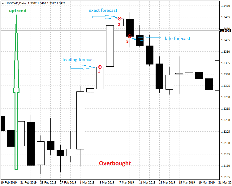
Fig.1. Ending trend forecast types, depending on the accuracy of identifying the overbought zone
Fig. 1 shows three red points obtained using various indicators to detect the overbought zone. Points from left to right: 1 — early forecast, 2 — accurate forecast, and 3 — retard forecast.
Obviously, "hitting" the trend extremum (accurate forecast of the ending trend) is a perfect market exit scenario if you have an open position. Therefore, the accuracy of forecasting the overbought/oversold zones, as related to that extremum, directly affects the efficiency of trading on financial markets.
We are going to consider this topic in more details below and evaluate the consequences of hitting the overbought/oversold zones in trading — both at entering and exiting the market. We'll start with the consequences of entering the market when in such zones.
Consequences of Entering the Market When in the Overbought/Oversold Zone
What consequences may a trader expect when entering the market in such a zone? Using a visual simplified analysis, appearance of an overbought/oversold zone is often associated with the presence of correction within the current trend. Therefore, let us consider the following options for the sequences of entering the market.
Option 1. There is no trend correction, or it is (subjectively) insignificant (which does not lead to the trend reversal yet). For analysis, we use points 1 and 2 in Fig. 1 (we don't consider point 3, since it is in the trend reversal area).
Consequences:
If the entry in in the trend "tail" and coincides with the direction of that trend, then everything depends on the residual amplitude value of the trend. If the residual amplitude is small (no one can guarantee a sufficient amplitude in the trend "tail"), then the profit value may turn out to be negligible or zero, or even negative, depending on how promptly the trader acts or how accurate the position closing signal is.
If it is about larger frames, such as D1 or higher, the situation there is not so definite, since the residual amplitude may turn out to be sufficient for short-term strategies, exactly because the candlestick amplitude is considerably larger there than in smaller timeframes. One such situation is point 1 (Fig. 1, early forecast of the overbought zone). Residual amplitude value of the uptrend turned out to be about 100 points (classical points in the 4th decimal place), which could be sufficient for obtaining profit, provided that you have entered with Buy at that point. However, it should be understood that we are viewing historical data in Fig. 1, while in a real situation, this point will be the last available point of the current trend at that moment, and it cannot be foreseen how early this signal will be and what the real residual amplitude of the trend will be. Moreover, a complex analysis on multiple timeframes will be required, since the larger timeframe signal, in this case, is just a preliminary signal and, to reduce risks, analysis on smaller timeframes is required, which is most frequently difficult for novice traders.
If the Buy entry is at point 2 (Fig. 1, accurate forecast of the overbought), the result will be negative, since this point is immediately followed by the reversal. Here, reasoning is similar to that in the preceding example.
If you enter in the trend "tail," but against that trend, your risk is elevated, in any case: If the trend continues, it will lead to a loss, while for a reversal, additional confirmations will be required, such as the activity of the reverse movements of price, which are, conditionally, yet not available. As an example, the Sell entry at point 1 or 2 (Fig. 1). If the Sell entry is at point 1 (early forecast of the ending uptrend), then, in this case, there is a considerable residual amplitude of the uptrend (about 100 points). Since StopLoss hardly exceeds this value, the position will be closed by it, with a loss. If the Sell entry is at point 2 (Fig. 1, accurate forecast of the ending uptrend), then the situation is perfect, since it is the end of the uptrend and, respectively, the very beginning of the downtrend.
Option 2. If there is a considerable correction of trend within this scale and the reverse price impulses are active, then, therefore, there is an increased probability of the trend reversal.
But what is a "considerable correction"? Of course, the notion of "considerable correction" is the subject of fuzzy logic, since there is no unique value of the correction depth, at which the trend will inevitably continue. There is only a range of values. For example, for the correction depth value below 20% (it's the range from 0% to 20%), it is highly probable that the trend continues. However, in practice, we can see that the trend also often continues after a correction of 50% and even 62%. Nevertheless, the correction of over 62% can (conditionally, of course) be considered a critical range of values, where the probability of the trend reversal increases rapidly.
Consequences:
If you enter within a deep correction and in the trend direction, your risk is elevated, in any case. If the trend still does not cope with the correction and the latter one translates into the opposite trend, there will be a loss. For the trend to still withstand the correction and continue in the same direction, you need very heavy additional confirmations with the current dynamics, such as new impulse activity in the trend direction, which is, conditionally, not yet available.
If you enter within the deep correction of this trend, but against the trend, risk is also elevated, in any case: If the trend continues, there will probably be a loss, while additional confirmations are required for the complete reversal, both the deep correction and the obvious activity of the reverse price movements that, conditionally, are not yet available.
Conclusions on Options 1 and 2:
Thus, entering the market when in an overbought/oversold zone, based on the signals of conventional indicators, both in and against the existing trend, is quite a risky strategy, since "there is not much of the trend left," and the accuracy of identifying such zones using conventional indicators is not high, which can additionally reduce the used residual amplitude of the trend. One single indicator can form either early or retard signals in different market situations (you can see that in ant chart of any financial instrument). At the same time, the smaller the timeframe, the higher the risk, since in absolute terms, the amplitude of smaller timeframes candlesticks (therefore, the absolute value of the residual trend amplitude) is smaller than the similar amplitude of candlesticks at higher timeframes, which is inevitable due to the different scales of price movements in the charts of different timeframes).
Let us consider a curious particular case of how the levels relate to each other ragarding the extremum of fractal that completes the trend. This is a situation where there are two entries in the trend direction at the same price level — the first entry at the point of the early forecast of the ending trend (to the left of the trend high), while the second entry is in the retard forecast area (to the right of the trend high).
Let's ask ourselves: Which entry is safer, if both entries are made at the same price level, but at different sides of the ending trend extremums (at different times)? Let us consider the example in Fig. 2:
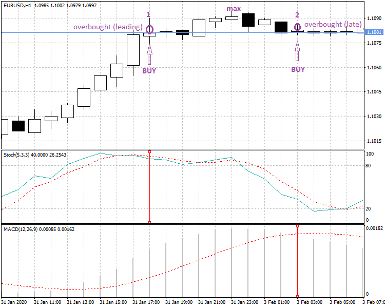
Fig. 2. Efficiency of Entering the Market at the Same Level, But at Different Times
Fig. 2 shows two entries at the same level, but at different times:
Point 1 — Buy entry (early forecast point of the ending trend, the overbought signal of the Stochastic indicator with default settings),
Point 2 — Buy entry (retard forecast point of the ending trend, the oberbought signal of the MACD indicator with default settings),
max — extremum of the local uptrend.
Fig. 2 shows that, despite the fact that the entries are at the same level, the entry at the ending trend early forecast point (Point 1) is safer, since there is still no reverse movement, and there is a reserve of the residual trend amplitude; therefore, losses are hardly probable (at least, when using short-term strategies). At the same time, an entry made in the area of the ending trend retard forecast (Point 2), though at the same level, is less safe, since, due to the retarding signal of the indicator, the price has already got into the correction (i.e., reverse movement) area; therefore, the loss probability is higher.
By all means, there are many market entering strategies and tactics that use the overbought/oversold zones (both in and against the trend direction). However, it is necessary to take the following into consideration: For an entry against the trend, you have to have some"watertight" non-technical (fundamental or news-based, for instance) external factors at hand to venture into such a nonstandard trading decision.
Evaluating Losses Related to the Risk of Opening a Position in Overbought/Oversold Zones
Let us put our theoretical conclusions to the test, exemplified by testing an Expert Advisor. Let us use an EA based on my preceding article: How to Reduce Trader's Risks (EA Reduse_risks, a version for MT5).
Our task is to use a particular case for evaluating possible losses related to the risk of entering within the overbought/oversold zones. To minimize the probability of entering within an overbought/oversold zone, let us use the algorithm of anchoring to the impulse beginning that is usually the local trend onset. We will discuss the algorithm itself later. So far, we are interested in the EA test results — first, the test using the module of anchoring to the trend onset (we reduce the probability of entering within an overbought/oversold zone), then the test with that module disabled (we remove protection represented by such anchoring, which increases the probability of entering within these zones — in the trend "tail").
Let us test the worst scenario to be as realistic as possible. We will intentionally take an example, in which the initial profit result is negative.
First Test Results (General Results and Balance Chart):
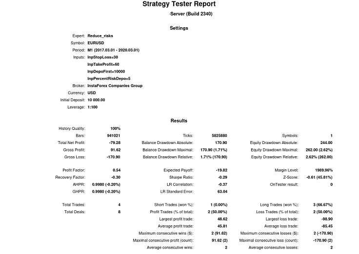
Figure 3. General test results with the enabled module of minimizing the risk of entering within an overbought/oversold zone

Figure 4. Balance/deposit chart with the enabled module of minimizing the risk of entering within an overbought/oversold zone
Fig. 3 and 4 show the results and the chart of the first test, in which the module of minimizing the risk of entering within an overbought/oversold zone was enabled. Don't let the lack of presence in the first test faze you, since, first, we are using an EA intended for our studies, not for real trading. Second, it is important to us what consequences can be anticipaed at this worst scenario.
Let us now disable the above protective module and test the EA.
Second Test Results (General Results and Balance Chart):

Figure 5. General results with the disabled module of minimizing the risk of entering within an overbought/oversold zone

Figure 6. Balance/deposit chart with the disabled module of minimizing the risk of entering within an overbought/oversold zone
Fig. 5 and 6 show the results of the second test, in which we have intentionally disabled the module of minimizing the risks related to opening a position within an overbought/oversold zone.
Let us compare the results of these two tests by some important parameters and display them in the following chart:
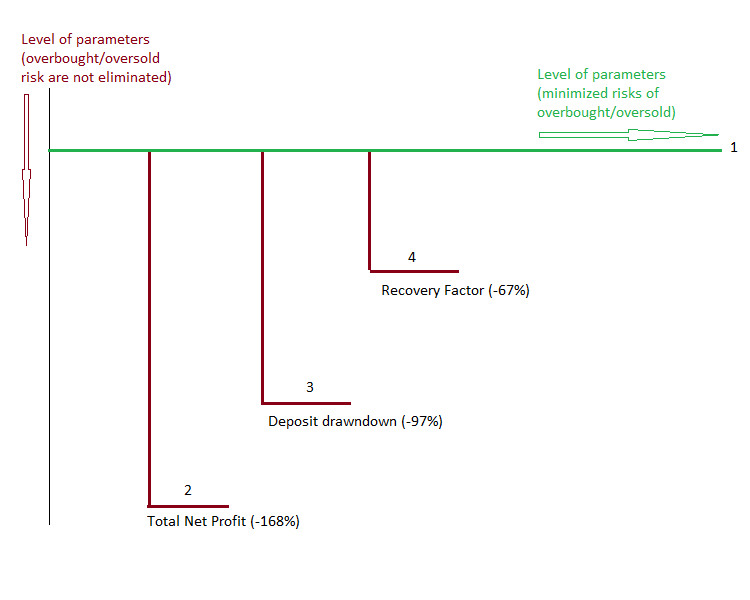
Figure 7. Chart of worsening parameters (trading efficiency) when ignoring the risks of entering the overbought/oversold zones
Fig. 7 shows the results of the first test — it is level 1 (a single starting level for all parameters), while the second test results are levels 2, 3, and 4. As we can see in the chart (test 2 as opposed to test 1), ignoring the risk related to opening a position within the overbought/oversold zones leads to adverse consequences — in this case, important indicators have considerably worsened as compared to the first test results. It does not matter that they were negative initially; it is important that they have considerably worsened as compared to the initial indicators:
"1" — Test 1 results, basic level (for each parameter obtained with the risk minimizing module enabled), with respect to which the indicators of test 2 have changed.
"2" — General traing result, worsening by 168%.
"3" — Deposit drawdown (while the maximum drawdown value is growing), worsening by 97%.
"4" — Recovery factor, worsening by 67%.
Thus, we have learned by practice that, if we don't take some special measures, then, considering the unsteadiness of market, some entries will get into an overbought/oversold zone, worsening the financial outcomes of trading.
Below we will consider the consequences of exiting the market (closing the existing open positions) in the overbought/oversold zones.
Consequences of Exiting the Market When in the Overbought/Oversold Zone
If entering the market in the overbought/oversold zones bears great risks (and, therefore, is unconditionally harmful for a trader), then exiting the market (closing an existing position) in such zones is rather helpful, since it reduces investment risks. Everything definitely depends on the indicator triggering accuracy. We have already learned earlier that the closer the exit point to the trend extremum (both by time and by amplitude), the lower the risks. Factors of time and amplitude are interrelated within a specific trend/correction section: If a point is closer to extremum by time, then it will also be closer to this extremum by amplitude (considering, of course, the chart line slope toward the time axis).
Let us consider the above, exemplified by oversold:
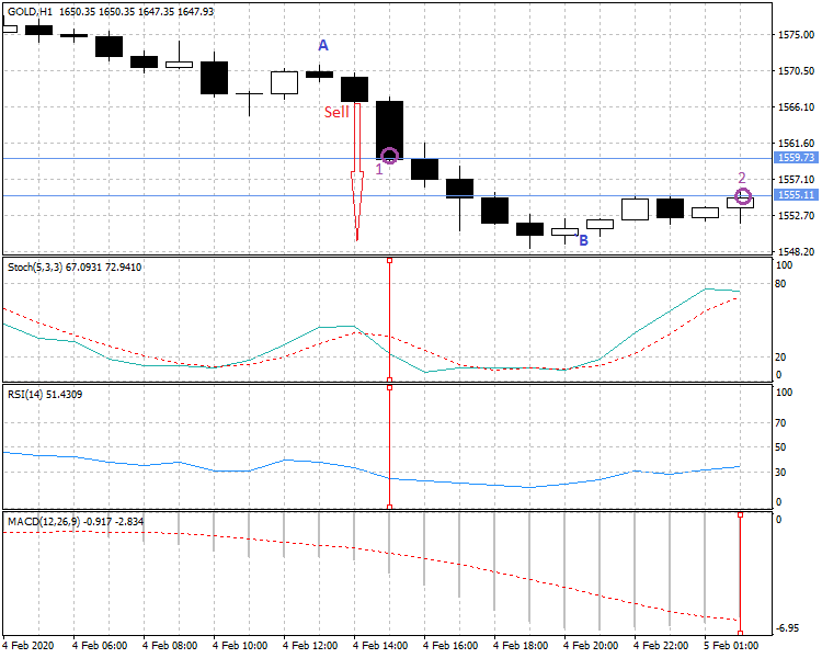
Figure 8. Closing a position within an oversold zone by different indicators
Fig. 8 shows two options of closing a Sell position, where:
(A-B) –downtrend amplitude,
red arrow starting point — the Sell entry point (a conditional entry immediately upon forming a fractal supporting the price moving down),
Point 1 — the point of closing a Sell position by indicators Stochastic, RSI (early forecast of the ending trend), and
Point 2 — the point of closing a Sell position by indicator MACD (retard forecast of the ending trend).
As we can see by historical data, exiting the market at point 1 appears to be premature - as a result, we obtain about 50% of the highest possible profit, while retarding exit will give us about 70% of the highest possible profit. In practice, it means that a retarding signal may turn out to be more profitable, if it is closer to the ending trend extremum, than an early signal.
The problem is, however, that we can compare the efficiency of these two signals on historical data, that is, only where the trend has already reversed. We won't be able to use the 1st signal at that time anymore. Therefore, in a real situation we will:
— Either use the 1st signal immediately upon its appearance (closing the position at point 1 in Fig. 8),
— Or ignore the 1st signal (using, for instance, indicator MACD as a filter — it does not support the actions of indicators Stochastic and RSI at point 1) and close the position at point 2 in Fig. 8.
Conclusions:
Closing a position (exiting the market) in an overbought/oversold zone is useful, since investment risks are reduced. Namely.
If we close based on the early forecast of the ending trend, then we will get additional profit at the price slippage, since there is some "operating range" in the trend (residual trend amplitude). In case of closing a position based on a retard forecast of the ending trend, everything depends on the distance from the trend extremum. The farther the market exit point from the trend extremum (that is, the stronger the correction), the worse the trading results.
Thus, the trading results will depend on the action algorithm, by which trader will use the signals of indicators (if any at all) to exit the market. However, the majority of traders on financial markets use indicators in their trading to a greater or lesser extent.
Further, let us consider pros and contras of conventional indicators in searching for the overbought/oversold zones. Let us start with those available in popular trading terminals.
Pros and Contras of Using Conventional Indicators to Detect Overbought/Oversold Zones
Traders use various indicators to detect the overbought/oversold zones. We turn our attention to some of them, namely: RSI, Stochastic, Bollinger Bands, MACD, and Momentum. We will see below that the accuracy of those indicators is low — their signal are often retarding, the delays being able to become critical for a specific trading situation.
First of all, quite a sloven work of conventional indicators is caused by the random starting point in computations by the formulas underlying the algorithms of indicators. This is due to the fact that the calculation period in the formulas is a fixed value. However, the real market fluctuations have a period, the value of which constantly changes even within a time frame. Due to the lack of taking such market dynamics features into account, using conventional indicators results in a bad accuracy of registering the onset of an overbought/oversold zone, which only sometimes coincides with the real end of the financial instrument price fluctuations. For this very reason, algorithms based on such indicators do not usually allow obtaining a stable profit within a considerable testing segment. We are going to test the above indicators on the trends of four different types:— Steady trend,
— Active trend,
— Mixed trend (for example, steady with some active elements), and
— Sideways.
Since we don't know in advance which exactly indicator turns out to be efficient at the moment, we will observe how all indicators work in group, regarding the trend type. Results of a group of indicators working to detect the overbought/oversold zones on the trends of all types will be considered by particular examples - first, with default settings. Since we know from our experience that the accuracy of conventional indicators is low, we will try to somehow improve this (group) accuracy by changing the indicator settings, i.e., we will use some new settings. then we will form the logic of such settings, using well-known analytical tools.
Setting Up a Group of Indicators Using the Values of Fibonacci Series
Traders widely use the values of Fibonacci series to identify important price levels, such as corrections or extensions, and as the fixed values of the calculation periods for various moving averages.
Therefore, it will also be quite logical to use the values of Fibonacci series to set up a group of conventional indicators.
Logic of changing the settings of indicators: To enhance the accuracy of detecting the overbought/oversold zones, it is necessary that the signals of indicators are closer to the end of a local trend, i.e., closer to the last fractal extremym of the trend. Considering that the signals of indicators may be both early and retard regarding that extremum, it is practically necessary to improve the "density of hits" of the indicators, the trend extremum being the target. For this purpose, we will change the settings of indicators. These, of course, will almost be intuitive settings based on visual estimates. Nevertheless, we will still apply some logic - we will use the closest (regarding the standard settings) values of Fibonacci series to set up the values of the calculation periods of indicators. Moreover, where necessary, we will use a price type that we need and that is used in the indicator computations. We will also try and fit these new settings into the features of particular indicators.
Let us consider the new settings for each indicator in the group, taking the above logic into account.
That "Restless" Stochastic: Analyzing the Indicator Formula
Indicator Stochastic: Indicator Stochastic (an oscillator) is one of the most "dexterous" ones, which often leads to extremely early signals. Therefore, let us slow it down a little. For this purpose, let us change the "slowing" parameter by setting 5 instead of 3. Why 5? This is the closest number of Fibonacci series upwards. This results in some smoothing the Stochastic chart with non-critically slowing down its response to price changes. We have brought Stochastic "to its senses", having reduced the probability of early signals in detecting the overbought/oversold zones. Let us look inside this indicator and try to analyze its mathematical model. The indicator has two curves (components) — a fast one (%K) and a slow one (%D).
Formula of the fast component of indicator Stochastic:
%K=((C- min)/(max - min))*100;
where:
C — the last close price,
min — the lowest price traded over the period of “n” preceding bars,
max — the highest price traded over the same period (“n” preceding bars),
%K — current value of the fast component of Stochastic.
%D is the moving average regarding %K with a small smoothing period. Various types of smoothing can be used, such as simple, exponential, smoothed, and weighed. This is the slow component of the indicator.
Parameter "slowing" (that we have previously changed) affects the frequency of signals appearing: The larger the parameter value, the fewer signals of the indicator near the extreme values.
An important signal of indicator Stochastic is the crossing of curve %K regarding curve %D. Curve %K is faster (more sensitive) than curve %D, since the latter one is a derivative of the former one. Another important signal is the fact that the indicator lines are beyond the level channels 30-70 (or 20-80) of the indicator to estimate the overbought/oversold states. As to recommendations on using those signals, they may differ depending on sources in traditional analysis. Therefore, traders use them in different ways, depending on their personal preferences and experiences.
Let us study the mathematical model of this indicator. What are the pros and contras of such an algorithm? Its analytical model is quite simple; this is what the indicator does:
▪ Finds in history (at a certain, fixed search depth) the price high and low and identifies the maximum price amplitude at the given depth in the quotes history (max - min),
▪ Finds the current amplitude regarding the same low (С — min),
▪ Then it finds the ratio of the current amplitude to the maximum amplitude (this exactly is %K, the fast component of the indicator), and
▪ Constructs the moving average of the %K values (this exactly is %D, the slow component of the indicator).
What are the pros of such a model?
In fact, indicator detects the share taken by the current amplitude regarding a certain reference amplitude. Basically, a good approach, provided that the reference is correct.
What are the contras?
The main disadvantage is that the reference, regarding which the calculations are made (max – min), is not quite correct, an dhere is why. Basic boundaries of amplitudes in the charts of financial instruments are fractals. And these are fractals (and processes among them) are the important indicators of the market dynamics. Therefore, a more logical reference would probably be the price amplitude between the differently directed fractals (i.e., the preceding local trend). In Stochastic (as well as in all other conventional indicators), the fractal nature of the market is not practically taken into consideration. Fractals (candlesticks of fractals) are considered in their algorithms alongside other candlesticks ("like all"). However, as a well-known character of a well-known movie said: "We are brothers, but we are not equal." We have already seen by an example (test results in Fig. 7), that acting without anchoring to the fractal level worsens trading outcomes. This means that the candlesticks of fractals really matter.
From ignoring the fractal nature, the following situation occur: At a certain random depth in the quotes history, a certain amplitude is measured and then used as a reference (inside the algorithm of the indicator). Is it correct? It is a matter for a greater discussion, since it relates to global issues, such as what an elementary structure is for analyzing the dynamics of market prices (this, however, is beyond the scope hereof).
Summary: Stochastic, in general, is a good indicator. Even though it does not take fractal nature into consideration (but this is a "systematic" problem of traditional analysis), the indicator is quite savvy and sensitive. This is not only achieved due to its algorithm (comparing the amplitudes is a correct approach, in general), but also due to its standard default settings (a small depth of data search and a moving average with a smaller calculation period are used), which, in fact, determines its good sensitivity.
We will also consider other indicators.
Indicators Momentun and RSI:
Here, instead, the task is to improve sensitivity, since these indicators have a considerable default calculation period of 14. Let us use the above methods here. For this purpose, we will reduce the calculation period value of the indicators (use 8 instead of 14). Why 8? We reduced the period value down to the nearest Fibonacci number (ignoring 13 as number that is too close to 14 and would not practically change anything) to obtain earlier signals from indicators. At the same time, to smooth the charts of indicators, we changed the price type used in computing the indicators: We use the typical price instead of the close one. Why typical price? Because it is better balanced than the close price. As a result, RSI produces fewer false responses around important levels 30 and 70, while indicator Momentum provides better response to considerable corrections regarding the important level of 100. Why do we consider the settings of two absolutely different indicators at the same time? Just because, in this case, their settings coincide, nothing more, although the algorithms of those indicators are absolutely different, of course.
Indicator MACD:
Similarly, let us change the settings of this indicator. To reduce the lag of moving averages used in computing the MACD indicator, let us change the values of standard default settings for the nearest smaller values from Fibonacci series. As a result, instead of settings (12,26,9 by close price), we will obtain settings (8,21,5 by typical price), where the relevant MACD indicator parameters are from left to right: Fast ЕМА, slow ЕМА, and indicator SMA.
Indicator Bollinger Bands:
This indicator is based on the deviation regarding the moving average. Therefore, let us try to set up this parameter. Instead of the default value of 2, we will set the value of 1, while close price will be replaced by typical price. At the same time, there is no need for reducing the value of the indicator calculation period, which is 20 by default, since the indicator sensitivity gets considerably better without adding this. You can see that even at a simple visual control: At the new settings, the uttermost curves of the indicator become, in fact, like faster moving averages. At the same time, the indicator becomes more convenient for detecting trend segments — trends are now beyond all three curves of the indicator (the larger part of trends, not their smaller part as at previous settings). If the price is within such indicator, then this is either the very onset of the trend or the consolidation zones that can be neglected in identifying the trend as the zones of indefinite dynamics. Visually, it is much more convenient than to search for price bounces within the zone consisting of three curves of this indicator (at default settings).
Thus, we have decided on the settings. Of course, such settings are not a result of some classical, long-term optimization; these are just a logical prearrangement of the parameters of a group of indicators, aimed at increasing the "density of hits" to the overbought/oversold zones. Let us try and understand whether it is possible to somehow improve the work of a group of conventional indicators at searching for such zones.
For this purpose, as agreed, let's test how they work on different trend types, which will allow us to more completely evaluate the results for different dynamics of market prices.
Testing a Group of Indicators Detecting the Overbought/Oversold Zones on Different Trend Types
Since each indicator has several types of signals, let us deal with this matter first.
Selecting a type of indicator signals.
To identify the overbought/oversold zone, various types of signals from indicators are used. Since there are no strict rules in the conventional technical analysis, but just general recommendations on this matter, so each trader uses the type of signals they consider to be correct or convenient. Here are these types of signals:
▪ Intersection of two curves of the indicator,
▪ Crossing the signal level by one of the indicator curves (if the indicator has two curves),
▪ Crossing the signal level by the indicator curve (If the indicator has a single curve), and
▪ Reversal of the indicator curve (if the indicator has a single curve).
Using the indicator curve reversal seems to be profitable; therefore, it is recommended by some authors. However, such signals are often too early. Most importantly, the indicator curve reversal pattern itself may prove false (corrective, in a similar manner to the price chart correction). Therefore, we won't use this type of indicator signals herein (if even sacrificing accuracy sometimes). We are going to use the single-valued and more reliable, in terms of identification, signals of indicators: Those based on the intersection of curves or on crossing a critical level by a curve.
Trend types.
We have already named these trend types above (there are four of them in total). We will evaluate the work of indicators for each trend type separately — first, with default settings, then with the new settings we have already defined for each indicator in the group.
Accuracy in Detecting the Zones.
We will estimate the accuracy in detecting the overbought/oversold zones by the value of distance (in bars or in the time units of a particular timeframe) regarding the trend extremum time (absolute high for an uptrend or absolute low for a downtrend). The plus sign means an advancing signal, while minus means a retarding signal.
Note! Useful segment of the trend starts upon forming the supporting fractal, since such a fractal is the minimum sign of the future trend onset.
Detecting the overbought/oversold zones within a steady trend (with the default settings of indicators).
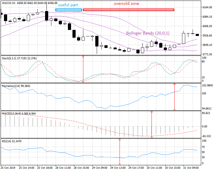
Figure 9. Indicators working on a steady trend to detect the overbought/oversold zones (standard default settings of indicators)
Fig. 9 shows the work of conventional indicators, i.e., Stochastic, Momentum, and RSI, with default settings (in this case, indicator Bollinger Bands is used with modified settings, but it is a help indicator here, just to visualize the downtrend: The trend is below the lower curve of that indicator).
Moments of the indicators triggering are shown using vertical red segments. As we can see, there is quite a large dispersion of indicators responses by time. We obtained the following error values as deviations (in bars) from the minimum fractal level of this local trend (plus means an advancing signal, minus means a retarding one): Stochastic "+12", Momentum "-7", MACD "-3", and RSI "+4".
Let us change the settings of the indicators.
Detecting the overbought/oversold zones within a steady trend (with the new settings of indicators).
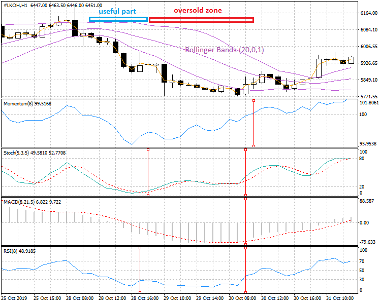
Figure 10. Indicators working on a steady trend to detect the overbought/oversold zones (new settings of indicators)
Fig. 10 shows the same indicators working, but with new settings.
Moments of the indicators triggering are shown using vertical red segments. As we can see, the dispersion on the indicators response values has significantly decreased with the new settings. We obtained the following error values as deviations (in bars) from the minimum fractal level of this local trend (plus means an advancing signal, minus means a retarding one): Stochastic changed from "+12" to "+11," Momentum "-7" to "-2," MACD "-3" to "-1," and RSI "+4" to "+12" (the signal is implicit, just a touch of the triggering level, so we can neglect it), and "-1." As a result, the value of the trend "coverage" has improved (see the extension of the blue horizontal zone in Fig. 10 as compared to Fig. 9).
Thus, regarding the steady trend type, in this case, the new settings of the indicators turned out to be more efficient than the default settings. Exception was one signal from RSI; however, it is not clear enough (the indicator curve did not cross the important level of 30, it only touched the level), so we can ignore it. At the same time, we will remember this spike of RSI (we will need this information later).
Let us perform a similar work regarding the active trend type and see whether the new settings will be efficient there.
Detecting the overbought/oversold zones within an active trend (with the default settings of indicators).
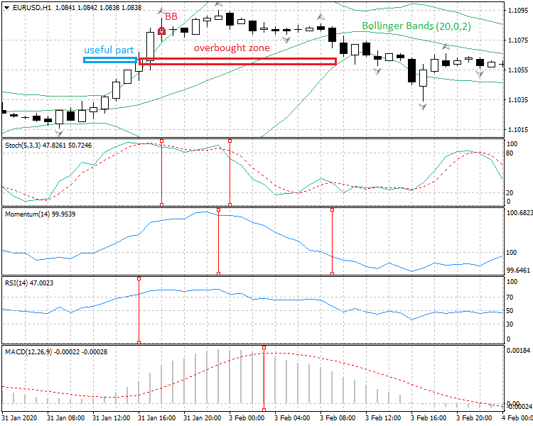
Figure 11. Indicators working on an active trend to detect the overbought/oversold zones (standard default settings of indicators)
Fig. 11 shows the work of conventional indicators, i.e., Stochastic, Momentum, RSI, and Bollinger Bands, with default settings (indicator Bollinger Bands is again used as a helper here, just to visualize the uptrend regarding the upper curve that indicator).
Moments of the indicators triggering are shown using vertical red segments. As we can see, there is quite a large dispersion of indicators responses by time. We obtained the following error values as deviations (in bars) from the minimum fractal level of this local trend (plus means an advancing signal, minus means a retarding one): Stochastic "+5" and "-1," Momentum "0" (bull's eye!) and immediately "-10," MACD "-4", RSI "+7," and Bollinger Bands "-10."
As we can see, the dispersion of responses (signals) of the indicators is quite large.
Let us change the settings of the indicators.
Detecting the overbought/oversold zones within an active trend (with the new settings of indicators).
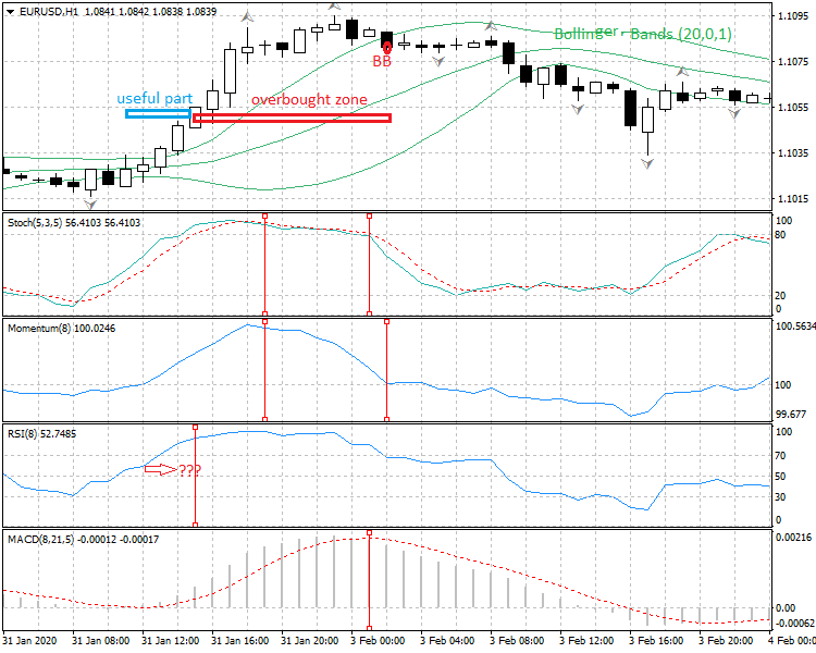
Figure 12. Indicators working on an active trend to detect the overbought/oversold zones (new settings of indicators)
Fig. 12 shows the same indicators working, but with new settings.
Moments of the indicators triggering are shown using vertical red segments. As we can see, there is quite a large dispersion of the indicators triggering by time, but most indicators "stick" by each other, while the accuracy of the signals of the group worsens RSI again. We obtained the following error values as deviations (in bars) from the minimum fractal level of this local trend (plus means an advancing signal, minus means a retarding one): Stochastic changed from "+5" and "-1" to "+4" and "-2," Momentum "0" and "-10" to "+4" and "-2," MACD "-4" to "-2," RSI "+7" to "+8," and Bollinger Bands from "-10" to "-3."
As we can see, almost all indicators have improved their results. Exceptions are indicators Stochastic and (especially) RSI — the signal of the latter one is out of the general picture of the signals from other indicators (shown as interrogative signs and red arrow in the figure).
Thus, regarding the active trend type, in this case, the new settings of the indicators turned out to be some more efficient than the default settings. Exception is, like with the steady trend, again, the "lone" signal of RSI. Let's make a note that RSI, again, did not show itself to be very good. It is this indicator, because of which the value of the trend "coverage" has not improved (insignificantly reducing the length of the blue horizontal area in Fig. 12 as compared to Fig. 11). Indicator Stochastic has insignificantly worsened the accuracy of detecting these zones. However, without considering RSI, the general situation has improved — the group accuracy in detecting the overbought/oversold zones has increased.
Let us raise the bar — perform the similar work regarding a more structurally complex trend, the mixed one (in which there are both a steady dynamics segment and an active dynamics segment).
Detecting the overbought/oversold zones within a mixed trend (with the default settings of indicators).
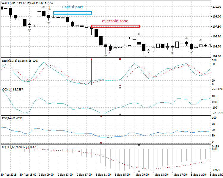
Figure 13. Indicators working on a mixed trend to detect the overbought/oversold zones (standard default settings of indicators)
Fig. 13 shows the work of the group of indicators on a mixed trend — the first part of the trend has relatively steady dynamycs, while the second one is active. For variety, let us also use indicator CCI. The results obtained for default settings: Stochastic: "+3" and "-3," CCI: "-3," RSI: "+1," and MACD: "-7." MACD provides the worst result in the group here.
Let us change the settings of the indicators.
Detecting the overbought/oversold zones within a mixed trend (with the new settings of indicators).
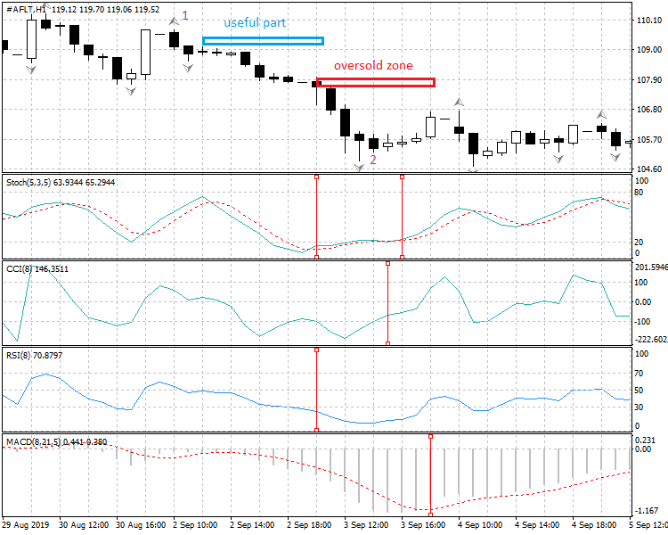
Figure 14. Indicators working on a mixed trend to detect the overbought/oversold zones (new settings of indicators)
Fig. 14 shows the same group of indicators working on a mixed trend, but with new settings. Obtain the results: Stochastic had "+3" and "-3," and the values remained the same, CCI: "-3" changed for "-2," RSI: "+1" changed for "-3," and MACD: "-7" changed for "-5." As a result, the general work efficiency has improved, except for RSI. Let us take note again: RSI has the worst result regarding the accuracy on the mixed trend, as in working on all preceding types of trends.
One more trend type, sideways, is remaining. Let us try to test how indicators work on this trend. Most likely, this will not be easy: In such a trend, many things depend on its amplitude. If its amplitude is considerable, then, in fact, each segment of this trend can be classified as one of the preceding ones. Therefore, it is basically hard to speak of the overbought/oversold zones in such a trend, since, if its amplitude is insignificant (within a specific scale), then the trend segments are very conditional. However, let's try and find discover something in this challenging option.
Indicators Working on Sideways (Default Settings)
Detecting the overbought/oversold zones within sideways (with the default settings of indicators).
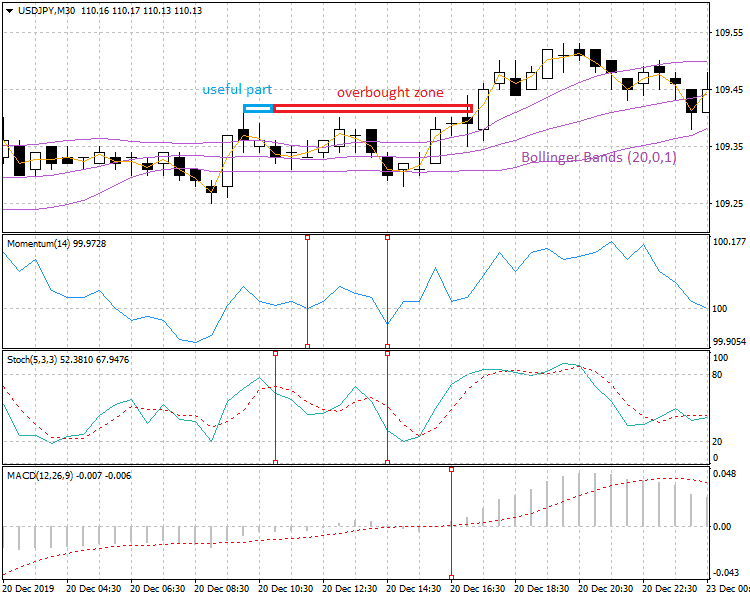
Figure 15. Indicators working on sideways to detect the overbought/oversold zones (standard default settings of indicators)
Fig. 15 shows how indicators with default settings work on detecting the overbought/oversold zones. In this sideways trend, the "useful" part (a light blue horizontal band) is useful for the Sell (not Buy) position, since the amplitude inside the channel is insignificant, and immediately upon the fractal supporting the up-movement, a reverse candlestick was formed and the local uptrend ()inside the channel) did not come about.
Let us change the settings of the indicators.
Detecting the overbought/oversold zones within sideways (with the new settings of indicators).
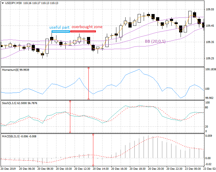
Figure 16. Indicators working on sideways to detect the overbought/oversold zones (new settings of indicators)
Fig. 16 shows how the same group of indicators work on detecting the overbought/oversold zones, with new settings. We can see that the useful part of the local trend (downtrend within the channel) has expanded, while the trend uncertainty area has rather decreased, which provides evidence of the enhanced accuracy of detecting such zones.
Now we have finished testing how the groups of indicators work on different trend types. It did not go unnoticed that RSI provided the lower quality of working. It was like an "enfant terrible" in the group. Let us figure out about the reasons for such a work of RSI.
What's Wrong with RSI? Analyzing the Indicator Formula
To understand the RSI operation principle, let us analyze the mathematical formula of this indicator.
Here is the formula of RSI:
RSI=100 - (100/(1+RS));
where:
RS — relative strength ratio (ratio of the average procie increment to the average price fall over the period.
RS=EMAup/EMAdn;
where:
EMAup — exponential moving average for all candles closed higher than the preceding candles, and
EMAdn — exponential moving average for all candles closed lower that the preceding candles.
Analysis of the indicator formula shows clearly why such an indicator works worse that the other ones on detecting the overbought/oversold zones on trends of different types (at least, in our examples). The reasons are as follows:
▪ First, price does not participate in calculating RSI as the primary market parameter (it uses the ratio of secondary parameters — moving averages, moreover, exponential ones), which unconditionally worsens the indicator accuracy. Moreover, separate ("patch") samples of the quotes array are used to form moving averages.
▪ Second, the logical core of the indicator (RS parameter) is "buried" quite deeply into the algorithm - it is in the denominator of the RSI calculation formula, its influence being weakened by the fact that the parameter is not used as it is, but is added by one. This, along with normalization used in the indicator (boundaries from 0 to 100), reduces the indicator sensibility.
Therefore, we can very conservatively assume that it is better to use RSI as an auxiliary filter rather than an alert indicator, while it would be more efficient to use other indicator for detecting the points determining the trading system signals. Why we suppose it "conservatively"? Just because an unconditional statement would need performing a large-scale investigation regarding this indicator (with different timeframes and financial instruments). However, I feel it my duty to warn the market players against any overconfidence of the unconditional efficiency of this widely advertized indicator (at least, as an alert one).
Well, we have studied the "mathematics" of RSI, so we will get back to the group work of our group of indicators now.
Results of Evaluating the Accuracy of Detecting the Overbought/Oversold Zones Depending on Settings and Trend Type
If you have noticed, we evaluated the accuracy of detecting the overbought/oversold zones, as well as the useful part of the trend, using a time scale (distance in bars regarding the trend extremum time). Now let's see how the accuracy of detecting such zones affects the efficiency of "covering" the trend amplitude.
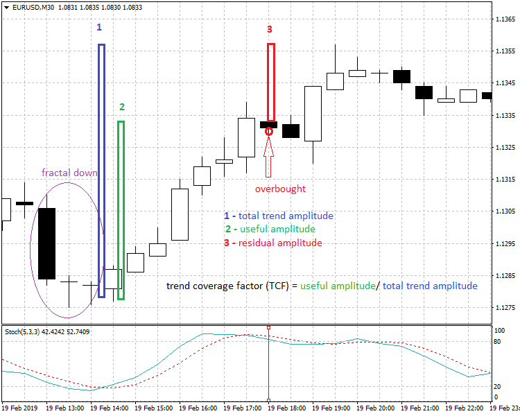
Figure 17. Indicating the trend amplitude coverage
Fig. 17 shows the EURUSD chart, and the Stochastic indicator with default settings is used as a working indicator to detect the overbought zone. Since, in this case, there is a local uptrend, then, therefore, we mean a Buy position:
This example shows how the accuracy of detecting the overbought zone affects the trading efficiency. Notation is as follows:
1 — full amplitude of the trend (of course, the supporting fractal amplitude — fractal down, in this case — is not taken into consideration, since the trend becomes "visible" (or rather slightly distinguishable) only upon forming this fractal),
2 — useful amplitude of the trend (it is the amplitude determining the profit, provided that we close the Buy position at a point highlighted by the red arrow), and
3 — residual amplitude of the trend (it is the amplitude hat is "lost," if the trader uses the signal of the Stochastic indicator as the overbought zone onset and closes the position).
From the formula shown in Fig. 17, we can see that the higher the accuracy of the overbought zone detection, the higher the trend amplitude coverage coefficient (and therefore, the higher trading efficiency).
It is clear that the more active the trend (i.e., the larger the angle of the trend deviation from the time axis, no matter whether it is an up- or downtrend), the more considerable the profit will be from enhancing the accuracy of detecting the overbought/oversold zones, since the amplitude of one candle (bar) in an active trend is broader than in other trend types. In practice, the largest part of the lifetime of markets are other types of trends (steady, mixed, or sideways) rather than active ones. Therefore, considering the trend type, gains in the accuracy of detecting such zones by the time parameter will not always ensure any remarkable gains in amplitude. Considering the dimensionality of such analysis (values of gains in amplitude depending on the accuracy of registering the zones in time),we will limit ourselves by the accuracy as related to the time factor. Moreover, we are analyzing the operation of a random set of indicators, not a specific trading system. And our task is to estimate the capability of this group of indicators regarding detecting the overbought/oversold zones, depending on the settings and the trend type.
Nevertheless, the formula shown in Fig. 17 can be used to evaluate the efficiency of any trading system as an additional parameter of standard estimation.
Let us assess the results of changing the accuracy of detecting the overbought/oversold zones by the group of indicators when modifying their settings (initially, we use the default settings, while the new ones are made based on the nearest numbers of Fibonacci series) by the time parameter (summirized for all types of trends).
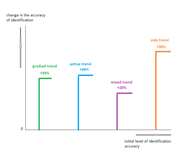
Figure 18. Curve of enhancing the accuracy of detecting the overbought/oversold zones (by a group of indicators) depending on the settings and trend types
Fig. 18 shows the curve of chaning (enhancing) the accuracy in detecting the overbought/oversold zones depending on the settings of indicators and on the trend type. Horizontal scale corresponds with the initial accuracy level (for the default settings of the group of indicators).
Vertical scale shows the values of accuracy changes (with the new settings of the indicators) regarding the initial level (with the default settings). Each trend type has its own color.
Green line shows changes in accuracy on a steady trend. Blue line shows changes in accuracy on an active trend. Violet line shows changes in accuracy on a mixed trend. Orange line shows changes in accuracy on sideways.
What conclusions can be drawn based on this graph? I don't think that we can draw any serious conclusions for the absolute values of enhancing the accuracy, like "if the trend is mixed, the accuracy grows slower for it than for any other trend types" (global studies are necessary for such statements). However, we can definitely say that the accuracy of detecting the overbought/oversold zones is basically higher with new settings (in this case, by at least one fourth, as compared to that with the default settings).
Conclusions on the Efficiency of Conventional Indicators Detecting the Overbought/Oversold Zones
We have seen in a specific context that with default settings, conventional indicators manifest quite a low accuracy when used to detect the overbought/oversold zones. In many cases, signals of the indicators are too early (which significantly reduces the profit due to losing the largest part of the trend amplitude) or significantly delay (which considerably reducesthe probability of obtaining any profits at all — due to the existing trend reversal).
We have found out that we should search for the reason for quite a sloven work of conventional indicators in their mathematical models that don't practically consider the nonstationary nature of the price movement processes. Algorithms of such indicators completely ignore the key factors of trend structures on financial markets, namely: They don't take the fractal nature of trend beginnings and ends into consideration and they don't extend the dynamics of changing the parameters of candles (they just gloss over them), of which trends consist, including in the areas of forming the overbought/oversold zones.
Instead, a random (not fractal) starting point is used for calculating the indicator values when computing by the formula underlying the algorithm of a particular indicator. As a result, calculating the indicator values does not start strictly from the trend onset, but amidst the current trend, or it covers a part of the preceding trend, which distorts the forecasting results significantly. This is due to the fact that the calculation period in the formulas of indicators is mostly a fixed value, each trader randomly changing the indicator calculation period value, i.e., the depth of using historical data, "to each their own."
However, market lives under its own laws: Real market fluctuations have a period (and a frequency as an inverse value), the value of which is not fixed, but changes continually even within a small time interval. In this context, anchoring to the trend onset appears to be reasonable.
Due to the lack of taking such "natural" market dynamics features into account, using conventional indicators results in a bad accuracy of registering an overbought/oversold zone, which only sometimes coincides with the real end of the local trend. For this very reason, automated trading systems based on such conventional indicators do not allow obtaining a stable profit within a longer testing segment.
Of course, trading systems without risk limits (StopLoss) don't count — they may sometimes manifest the unparalleled results of profitability, even when using conventional indicators, due to ignoring drawdowns. However, we cannot ignore risks in real trading, since such drawdowns will ealier or later consume trader's deposit if StopLoss is not used (my own experience of testing multiple different trading systems proves that).
To enhance the indicators operation aimed at detecting the overbought/oversold zones, we used a simple method without any pre-optimization and used (fixed) settings instead of the default ones. The new settings were made as follows: The setting parameter value was changed for the nearest values of Fibonacci series. Even such simple changes allowed us to enhance the accuracy of detecting the overbought/oversold zones by the "time" parameter by at least a quarter.
Based on testing results, we also analyzed the operation of two indicators (the best one and the worst one, in this case) in greater detail. In the in-depth analysis of the mathematical formulas of the above indicators (Stochastic and RSI), we identified the factors affecting the operation quality of those indicators.
For example, it was found that the mathematical model of Stochastic ensured good performance, even with default settings.
At the same time, it was shown that the operation of the well-known RSI as a signal indicator was challenging, exactly due to its mathematical model. Therefore, despite its wide popularity, this indicator may have some operational constraints (although not exclusively in detecting the overbought/oversold zones, but in its general operation). Analysis of the mathematical model showed that it would be logical to use RSI as a general filter, i.e., we should use the range of the indicator values rather than crossing the indicator levels at certain points (the indicator model does not basically allow ensuring any high sensitivity).
New Approaches to Enhance the Efficiency of Detecting the Overbought/Oversold Zones
Well, what should actually be the novelty of approaches to detecting the overbought/oversold zones? Let us summarize general requirements. Since we discussed the need for taking fractals (trend onset and end) into consideration and the necessity of analyzing the elements within the trend, we can talk of fractal-candle analysis.
General Requirements for the Indicator Algorithm to Detect the Overbought/Oversold Zones Using Fractal-Candle Analysis
Considering the disadvantages of conventional methods used for detecting the overbought/oversold zones, the following can be recommended:
▪ A valid reference starting point should be selected, not a random one (as it is the case in conventional indicators), to calculate the function values of any indicators (at any time). What is that starting point? It is undoubtedly the supporting fractal extremum. Why fractal extremum? Because exactly such levels are the explicit marks of the market dynamics, which are perceived by the market players as reference times (to set a StopLoss, for instance). We have already mentioned above that it is the lack of such reference points in the calculation algorithms of conventional indicators that reduces the accuracy of detecting the overbought/oversold zones.
▪ Calculation period of conventional indicators is a fixed value, while real price movements have the continually changing frequency value (and, therefore, the calculation period value) of fluctuations. This lead to the inadvertent errors of such indicators when detecting the overbought/oversold zones.
▪ In accordance with the impulse equilibrium theory, candlestick is not a full-fledged elementary structure for analyzing the market dynamics, while the conventional candle analysis patterns are not always suitable for analyzing, since candlestick is an element of such patterns. Cadnlestick, despite the ease of displying information by it, has major defficiencies, such as: Important fractal levels are not visible inside a candlestick. Moreover, Open and Close candle levels are practically never fractal, which requires some additional analyses of price changes after those points. To reduce the role of such negative factors to at least some extent, the following must be done when performing candle analysis within the trend:
Detailed analysis of the candle "body" / candle amplitude ratio for each candlestick (this characterizes in a simplified manner the total activity of the process, as a microtrend, inside the candle),
Analysis of how correction inside a candle correlates with its total amplitude (this characterizes in a simplified manner the dynamics of the process at the latest stage of forming a candle, before the onset of forming the next candle of the trend), and
Comprehensive multiscale approach, namely: Since the Open and Close levels are not fractals, we need an additional precise analysis of dynamics on a smaller timeframe - both to analyze the activity at the latest stage of forming and closing (the preceding larger) candlestick and to analyze the activtity after opening the next candlestick.
▪ Regarding the structure of an analytical system to detect the overbought/oversold zones.
According to the factors of the impulse equilibrium theory, the algorithm of any analytical or trading system must be multimodal, since the price movement of any financial instrument is a complex nonstationary process that cannot be described by a simple algorithm. The above is also completely true of the algorithm of detecting the overbought/oversold zones (any conventional indicator algorithm always represents the simplified modeling of market dynamics). In detecting such zones, there can be many patterns of dynamics. Therefore, a more logical solution of the problem of detecting the overbought/oversold zones is a common algorithm consisting of multiple variations (relatively simple algorithms) unified by the logical "OR" function. Why should you use logical OR? Because each variation (of the situation characterizing the onset of such zone) can theoretically be formed with the same probability, but we don't know in advance what exactly variation will be formed.
We have shown above that the combination of fractal analysis and candle analysis can be the most efficient option for modeling the market dynamics. Of course, this is not about the classical patterns of candle analysis. It is about some newer solutions in this area.
Thus, let us proceed to the specific methods of solving our challenging problem.
Method Related to Identifying the Signs of the Trend "Slowdown"
In our preceding article (How to Reduce Trader's Risks), we showed that a more accurate way of detecting the overbought/oversold zones (as compared to conventional indicators) was the identification of slowdown signs within the current local trend by the following criteria:
— Shortening the distance (amplitude) between the neighboring fractal support levels (we need three fractals to compare the amplitudes of two neighboring segments),
— Increasing the correction depth inside the candlestick and reducing the candle "body" (intra-candle analysis), and
— Changing the direction of shifting the candle pivot regarding the pivot of the preceding candle (three candles are needed to compare these levels).
There is one more method — the one using anchoring to the trend onset (as a starting point for further forecasting the overbought/oversold zones). Let us consider the algorithm of such anchoring.
Algorithm of Anchoring to the Trend Onset
Impulse equilibrium theory shows that one of the important components in an analytical or trading system is the module of anchoring to the onset of wavelike movement, i.e., to the local trend onset. We learned by a specific example (chart in Fig. 7) above that disabling this module, i.e., ignoring the risks related to "hitting" the overbought/oversold zones, reduces the efficiency of a trading system considerably. Any indicator is an analytical system that should take this into consideration. It is the lack of such anchoring in conventional indicators that is the core factor of their inaccurate operation.
How to use this parameter in detecting the overbought/oversold zones? This anchoring seems to be necessary, first of all, to forecast the trend onset for entering the market. However, anchoring to the trend onset turned out to be helpful in detecting the above zones. For this purpose, we have to keep our distance from the local trend onset, and this will enhance the probability of "hitting" the movement "tail" (and this is exactly what we need to detect the overbought/oversold zones).
Fig. 19 below shows the module of anchoring to the trend onset (as part of Expert Advisor Reduce_risks for MT5).
In this case, a sign of the trend onset to be forecasted is the intersection of moving average and the candlestick in history: MA8 for M1 and MA5 for M15. Calculation periods of moving averages were taken from the values of Fibonacci series.
Please note that the intersection (of the candlestick and the MA) on the M1 timeframe is not limited by one bar in history. It is set by the logical OR - either on the preceding bar or on the 2nd bar in history, or on the 3rd bar in history (on M1). For M15, in this case, a single intersection option is available, i.e., on the preceding bar in history. This set of potential options makes it possible to take into account the multi-variant real market situations associated with the development of a local trend relative to such an intersection.
The example is shown for entering the market (using such algorithm, we reduce the probability of getting into an overbought/oversold zone). The algorithm is universal — it can be used for both up- and downtrends, since the algorithm does not (intentionally) take the directions of candlesticks into account.
Let's consider a code fragment of the module of anchoring to the trend onset (MQL5-version):
int            handle_iMA_M1_period5;        // variable for storing the handle of the iMA indicator
int            handle_iMA_M1_period8;        // variable for storing the handle of the iMA indicator
int            handle_iMA_M1_period13;       // variable for storing the handle of the iMA indicator
int            handle_iMA_M1_period60;       // variable for storing the handle of the iMA indicator
int            handle_iMA_M15_period4;       // variable for storing the handle of the iMA indicator
int            handle_iMA_M15_period5;       // variable for storing the handle of the iMA indicator
int            handle_iMA_M15_period8;       // variable for storing the handle of the iMA indicator
int            handle_iMA_H1_period24;       // variable for storing the handle of the iMA indicator

...................................................................................................

 handle_iMA_M1_period5=iMA(m_symbol.Name(),PERIOD_M1,5,0,MODE_SMA,PRICE_TYPICAL);
//--- if the handle is not created
   if(handle_iMA_M1_period5==INVALID_HANDLE)
     {
      //--- tell about the failure and output the error code
      PrintFormat("Failed to create handle of the iMA indicator for the symbol %s/%s, error code %d",
                  m_symbol.Name(),
                  EnumToString(Period()),
                  GetLastError());
      //--- the indicator is stopped early
      return(INIT_FAILED);
     }
//--- create handle of the indicator iMA
   handle_iMA_M1_period8=iMA(m_symbol.Name(),PERIOD_M1,8,0,MODE_SMA,PRICE_TYPICAL);
//--- if the handle is not created
   if(handle_iMA_M1_period8==INVALID_HANDLE)
     {
      //--- tell about the failure and output the error code
      PrintFormat("Failed to create handle of the iMA indicator for the symbol %s/%s, error code %d",
                  m_symbol.Name(),
                  EnumToString(Period()),
                  GetLastError());
      //--- the indicator is stopped early
      return(INIT_FAILED);
     }


handle_iMA_M15_period5=iMA(m_symbol.Name(),PERIOD_M15,5,0,MODE_SMA,PRICE_TYPICAL);
//--- if the handle is not created
   if(handle_iMA_M15_period5==INVALID_HANDLE)
     {
      //--- tell about the failure and output the error code
      PrintFormat("Failed to create handle of the iMA indicator for the symbol %s/%s, error code %d",
                  m_symbol.Name(),
                  EnumToString(Period()),
                  GetLastError());
      //--- the indicator is stopped early
      return(INIT_FAILED);
     }

..........................................................................................................


    //--- minimize the risks associated with entering the overbought zone at the entrance to the market
      //--- binding to the beginning of a wave to reduce probability of an entrance in a overbought zone:
      //---    the beginning of a wave - not further three bars in the history of data (M1)
      bool beginning_wave_M1=
                             (arr_MA_M1_period8[1]>rates_M1[1].low && arr_MA_M1_period8[1]<rates_M1[1].high) ||
                             (arr_MA_M1_period8[2]>rates_M1[2].low && arr_MA_M1_period8[2]<rates_M1[2].high) ||
                             (arr_MA_M1_period8[3]>rates_M1[3].low && arr_MA_M1_period8[3]<rates_M1[3].high);
      //---    the beginning of a wave - on the previous bar of the senior timeframe (M15)
      bool beginning_wave_M15=
                              MA_M15_period5_1>rates_M15[1].low && MA_M15_period5_1<rates_M15[1].high;


...............................................................................................................


 if(amplitude_candles_M1 &&
         amplitude_candles_M15 &&
         amplitude_channel_M15 &&
         activity_previous_bar_M1 &&
         local_resistance_overcome &&
         beginning_wave_M1 &&
         beginning_wave_M15 &&
         ascending_direction_2nd_bar_M1 &&
         ascending_direction_previous_bar_M1 &&
         ascending_MA_5and60 &&
         hierarchy_of_three_MA &&
         current_price_is_higher_than_MA &&
         ascending_direction_of_the_previous_candle_M15 &&
         ascending_MA_period4 &&
         hierarchy_of_two_MA_M15 &&
         current_price_is_higher_than_MAperiod4_M15 &&
         current_price_is_higher_than_MAperiod24_H1 &&
         share_of_body_M15 &&
         restriction_of_depth_of_correction_M15 &&
         ascending_tendency_M15 &&
         existence_of_a_shadow_M15 &&
         share_of_body_M1 &&
         previous_candle_no_flat &&
         restriction_of_depth_of_correction_M1 &&
         ascending_a_tendency_M1 &&
         existence_of_a_shadow_M1)
Fig.19. Module of anchoring to the trend onset.
Fig. 19 shows the module of anchoring to the trend onset (as part of Expert Advisor Reduce_risks for MT5). Notation:
arr_MA_M1_period8[1], arr_MA_M1_period8[2], arr_MA_M1_period8[3] — moving average with the calculation period of 8, calculated on the preceding, the 2nd, and the 3rd bar, respectively, in the history of quotes (timeframe M1),
MA_M15_period5_1 — moving average with the calculation period of 5, calculated on the preceding bar in history (timeframe M15),
rates_M1[1].low, rates_M1[2].low, rates_M1[3].low, rates_M1[1].high, rates_M1[2].high, rates_M1[3].high — extremums of candlesticks on respective bars in history (teimframe M1), and
rates_M15[1].low, rates_M15[1].high — extremums of candlesticks on the preceding bar (timeframe M15).
Please note that, in the MQL5 version, the algorithm is executed in two steps: First, the conditions of anchoring to the trend onset are defined by separate variables (bool beginning_wave_M1 and bool beginning_wave_M15), then the values of those variables are validated in the "if" operator (By logical AND, they are highlighted in green).
Further, we will learn how anchoring to the trend onset can be used to detect the overbought/oversold zones.
Method Related to Distancing from the Trend Onset
Thus, we have identified the trend onset (it is a forecast, of course, since not every trend will really go any further). Now we have to see how this will be used to detect the overbought/oversold zones.
Here comes the comprehensive method combining the above solutions — anchoring to the trend onset and detecting the trend slowdown signs (after the anchoring point already). In our simplified version of using this method, a disadvantage will be that such indicator will look on even the very first correction as an overbought/oversold zone. Therefore, to reduce the likeliness of false signals from the indicator, we can use the following trend property:
Trend (more precisely, its active part) time is a finite value that, in most cases, does not exceed 10–15 bars for any timeframe (any financial instrument).
The important result is that:
The further the current price (in bars) will move away from the trend onset (approaching to the numbers specified), the higher the probability of the ending trend will be (and the higher the probability of the early stage of the ending trend to appear — and this will exactly be the overbought/oversold zone, depending on the trend direction).
Such reasonably distancing from the trend onset allows reducing the amount of false signals due to ignoring the nearest responses (related to anchoring to the trend onset).
Of course, in case of a sharp increase in the amplitude of prices moving against the trend, the factor of distance will be of less importance, and we will have to consider the types of risk related to reverse impulses (risk categories and the relevant algorithms are presented in my article titled How to Reduce Trader's Risks). These are the following risk categories: Risks associated with uncertainty of the price movement amplitude after a market entry and risks associated with a price collapse after a market entry.
Conclusions
Well, we've done with the first part of the topic: On Methods to Detect Overbought/Oversold Zones now. What's new we have learned?
▪ First of all, we have clarified the very concept of such zones, in terms of the nautre of price movement process, namely, its fractality.
▪ We have evaluated the consequences of entering the market within such zones and those of closing positions in such zones, based on assumption that these zones are a variety of a broader notion — zones of uncertainty (see for more details in the theory of impulse equilibrium).
▪ We considered how a group of conventional indicators works on detecting such zones with both standard and new settings (based on the nearest values of Fibonacci series). Testing was comprehensive, i.e., on trends of different types. Since the new settings were proposed based on theoretical assumptions, not on volumetric testing, they cannot be considered as strict recommendations for trading. At the same time, even such pre-studies have shown that using the values of Fibonacci seriesfor the settings of conventional indicators (for example, those nearest to the standard ones), in general, are a positive factor to enhance their accuracy, particularly in detecting the overbought/oversold zones. Therefore, such settings very well may be used as the initial values for the volumetric optimization of trading systems using conventional indicators.
▪ Having analyzed the mathematical formulas of some indicators in the group, we learned that not all indicators can be used as alerting ones. For example, mathematical model of RSI is unfortunately so that, if RSI were a thermometer, we would only see something ill-defined, like "it's warm/cool now," instead of an exact temperature value. The reason is that the algorithm of this indicator uses not primary data (market prices to be directly compared in some), but secondary data (moving averages). Moreover, these moving averages are also very specific, "cut-off" — not the entire sequence of prices within the selected range is used to calculate them, but just a sample from this sequence within the same range. Therefore, quite a well-founded assumption was formed that it would be more reasonable to use RSI as a general filter only, not as an alerting indicator. That is, it is more reasonable to use not the triggering times (where their curves intersect), but a broader range of the indicator values, having given the way to other indicators in selecting the response points. This fact may be interesting to many traders using RSI that is an "old stager" at traditional technical analysis.
▪ At the same time, we have learned that indicators, the algorithms of which analyze and drectly compare primary data (and, which is important, amplitudes of various sequential intervals in the chart), have a higher accuracy in detecting the overbought/oversold zones and better flexibility of / sensitivity to changing the settings. An example of such indicator is Stochastic, using which as an alerting indicator appears to be quite reasonable.
▪ Some new approaches were also proposed to enhance the accuracy in detecting the overbought/oversold zones. A complex fractal-candle analysis was proposed, namely: Algorithmically anchoring to the trend onset, distancing, and analyzing the dynamics of a smaller scale (each candlestick in the current trend is considered as an impulse from a smaller timeframe).
Implentation.
▪ The author's indicator to detect the overbought/oversold zones, developed based on the methods described herein can be found in the Market here.
▪ This article uses the algorithms of Expert Advisor Reduce_risks (MQL5 version by Vladimir Karputov) — the codes are attached hereto (set for timeframe M1).
EAs are described in detail in article titled How to Reduce Trader's Risks and here. IMPORTANT! This EA was developed for research purpose only and is not intended for real trading!
In the second part of the article On Methods to Detect Overbought/Oversold Zones, we are going to discuss the following topics:
▪ Pros and contras of using the conventional methods of detecting the overbought/oversold zones, using the following analysis tools:
- Adaptive moving averages,
- Fibonacci levels,
- Divergence,
- Chart patterns,
- and the opportunities of using the above methods.
▪ Issues of enhancing the efficiency of the above analytical tools.
Translated from Russian by MetaQuotes Ltd.
Original article: https://www.mql5.com/ru/articles/7782
 Probability theory and mathematical statistics with examples (part I): Fundamentals and elementary theory
 A system of voice notifications for trade events and signals
 Quick Manual Trading Toolkit: Working with open positions and pending orders
- Free trading apps
- Over 8,000 signals for copying
- Economic news for exploring financial markets
You agree to website policy and terms of use
I've enjoyed both articles, Reducing Risk and this one. In your articles, you reference Lower and Higher Time frames and use the Lower time frame of M1 for testing. As I am using H4, is it appropriate to change the references from M1 to H4 and M15 to D1 and do the constants of 200 and 300 need to be changed as well. In addition, you did not supply the additional include files to get the MQ5 versions to compile.
Hi, Interesting and informative. I am in learning mode and independantly of this article am using Aligator teeth etc which are based on Fabinchi numbers.
interested in
In the second part of the article On Methods to Detect Overbought/Oversold Zones, we are going to discuss the following topics:
Where is the second part please.